Introduction

In most presentations of Riemannian geometry, e.g. O’Neill (1983) and Wikipedia, the fundamental theorem of Riemannian geometry (“the miracle of Riemannian geometry”) is given: that for any semi-Riemannian manifold there is a unique torsion-free metric connection. I assume partly because of this and partly because the major application of Riemannian geometry is General Relativity, connections with torsion are given little if any attention.

It turns out we are all very familiar with a connection with torsion: the Mercator projection. Some mathematical physics texts, e.g. Nakahara (2003), allude to this but leave the details to the reader. Moreover, this connection respects the metric induced from Euclidean space.

We use SageManifolds to assist with the calculations. We hint at how this might be done more slickly in Haskell.

A Cartographic Aside

%matplotlib inline

/Applications/SageMath/local/lib/python2.7/site-packages/traitlets/traitlets.py:770: DeprecationWarning: A parent of InlineBackend._config_changed has adopted the new @observe(change) API
  clsname, change_or_name), DeprecationWarning)

import matplotlib
import numpy as np
import matplotlib.pyplot as plt

import cartopy
import cartopy.crs as ccrs
from cartopy.mpl.ticker import LongitudeFormatter, LatitudeFormatter

plt.figure(figsize=(8, 8))

ax = plt.axes(projection=cartopy.crs.Mercator())

ax.gridlines()

ax.add_feature(cartopy.feature.LAND)
ax.add_feature(cartopy.feature.COASTLINE)

plt.show()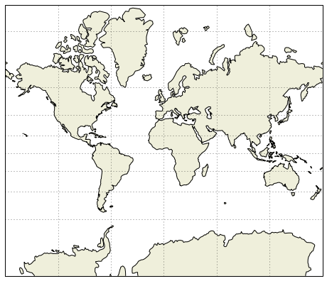

png

We can see Greenland looks much broader at the North than in the middle. But if we use a polar projection (below) then we see this is not the case. Why then is the Mercator projection used in preference to e.g. the polar projection or the once controversial Gall-Peters – see here for more on map projections.

plt.figure(figsize=(8, 8))

bx = plt.axes(projection=cartopy.crs.NorthPolarStereo())

bx.set_extent([-180, 180, 90, 50], ccrs.PlateCarree())

bx.gridlines()

bx.add_feature(cartopy.feature.LAND)
bx.add_feature(cartopy.feature.COASTLINE)

plt.show()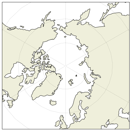

png

Colophon

This is written as an Jupyter notebook. In theory, it should be possible to run it assuming you have installed at least sage and Haskell. To publish it, I used

jupyter-nbconvert --to markdown Mercator.ipynb
pandoc -s Mercator.md -t markdown+lhs -o Mercator.lhs \
       --filter pandoc-citeproc --bibliography DiffGeom.bib
BlogLiteratelyD --wplatex Mercator.lhs > Mercator.html

Not brilliant but good enough.

Some commands to jupyter to display things nicely.

%display latex

viewer3D = 'tachyon'

Warming Up With SageManifolds

Let us try a simple exercise: finding the connection coefficients of the Levi-Civita connection for the Euclidean metric on $\mathbb{R}^2$ in polar co-ordinates.

Define the manifold.

N = Manifold(2, 'N',r'\mathcal{N}', start_index=1)

Define a chart and frame with Cartesian co-ordinates.

ChartCartesianN.<x,y> = N.chart()

FrameCartesianN = ChartCartesianN.frame()

Define a chart and frame with polar co-ordinates.

ChartPolarN.<r,theta> = N.chart()

FramePolarN = ChartPolarN.frame()

The standard transformation from Cartesian to polar co-ordinates.

cartesianToPolar = ChartCartesianN.transition_map(ChartPolarN, (sqrt(x^2 + y^2), arctan(y/x)))

print(cartesianToPolar)

Change of coordinates from Chart (N, (x, y)) to Chart (N, (r, theta))

print(latex(cartesianToPolar.display()))

$\displaystyle \left\{\begin{array}{lcl} r & = & \sqrt{x^{2} + y^{2}} \\ \theta & = & \arctan\left(\frac{y}{x}\right) \end{array}\right.$

cartesianToPolar.set_inverse(r * cos(theta), r * sin(theta))

Check of the inverse coordinate transformation:
   x == x
   y == y
   r == abs(r)
   theta == arctan(sin(theta)/cos(theta))

Now we define the metric to make the manifold Euclidean.

g_e = N.metric('g_e')

g_e[1,1], g_e[2,2] = 1, 1

We can display this in Cartesian co-ordinates.

print(latex(g_e.display(FrameCartesianN)))

$\displaystyle g_e = \mathrm{d} x\otimes \mathrm{d} x+\mathrm{d} y\otimes \mathrm{d} y$

And we can display it in polar co-ordinates

print(latex(g_e.display(FramePolarN)))

$\displaystyle g_e = \mathrm{d} r\otimes \mathrm{d} r + \left( x^{2} + y^{2} \right) \mathrm{d} \theta\otimes \mathrm{d} \theta$

Next let us compute the Levi-Civita connection from this metric.

nab_e = g_e.connection()

print(latex(nab_e))

$\displaystyle \nabla_{g_e}$

If we use Cartesian co-ordinates, we expect that $\Gamma^k_{ij} = 0, \forall i,j,k$ . Only non-zero entries get printed.

print(latex(nab_e.display(FrameCartesianN)))

Just to be sure, we can print out all the entries.

print(latex(nab_e[:]))

$\displaystyle \left[\left[\left[0, 0\right], \left[0, 0\right]\right], \left[\left[0, 0\right], \left[0, 0\right]\right]\right]$

In polar co-ordinates, we get

print(latex(nab_e.display(FramePolarN)))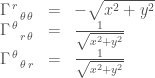

$\displaystyle \begin{array}{lcl} \Gamma_{ \phantom{\, r } \, \theta \, \theta }^{ \, r \phantom{\, \theta } \phantom{\, \theta } } & = & -\sqrt{x^{2} + y^{2}} \\ \Gamma_{ \phantom{\, \theta } \, r \, \theta }^{ \, \theta \phantom{\, r } \phantom{\, \theta } } & = & \frac{1}{\sqrt{x^{2} + y^{2}}} \\ \Gamma_{ \phantom{\, \theta } \, \theta \, r }^{ \, \theta \phantom{\, \theta } \phantom{\, r } } & = & \frac{1}{\sqrt{x^{2} + y^{2}}} \end{array}$

Which we can rew-rewrite as

$\displaystyle \begin{aligned} \Gamma^r_{\theta,\theta} &= -r \\ \Gamma^\theta_{r,\theta} &= 1/r \\ \Gamma^\theta_{\theta,r} &= 1/r \end{aligned}$

with all other entries being 0.

The Sphere

We define a 2 dimensional manifold. We call it the 2-dimensional (unit) sphere but it we are going to remove a meridian to allow us to define the desired connection with torsion on it.

S2 = Manifold(2, 'S^2', latex_name=r'\mathbb{S}^2', start_index=1)

print(latex(S2))

$\displaystyle \mathbb{S}^2$

To start off with we cover the manifold with two charts.

polar.<th,ph> = S2.chart(r'th:(0,pi):\theta ph:(0,2*pi):\phi'); print(latex(polar))

$\displaystyle \left(\mathbb{S}^2,({\theta}, {\phi})\right)$

mercator.<xi,ze> = S2.chart(r'xi:(-oo,oo):\xi ze:(0,2*pi):\zeta'); print(latex(mercator))

$\displaystyle \left(\mathbb{S}^2,({\xi}, {\zeta})\right)$

We can now check that we have two charts.

print(latex(S2.atlas()))

$\displaystyle \left[\left(\mathbb{S}^2,({\theta}, {\phi})\right), \left(\mathbb{S}^2,({\xi}, {\zeta})\right)\right]$

We can then define co-ordinate frames.

epolar = polar.frame(); print(latex(epolar))

$\displaystyle \left(\mathbb{S}^2 ,\left(\frac{\partial}{\partial {\theta} },\frac{\partial}{\partial {\phi} }\right)\right)$

emercator = mercator.frame(); print(latex(emercator))

$\displaystyle \left(\mathbb{S}^2 ,\left(\frac{\partial}{\partial {\xi} },\frac{\partial}{\partial {\zeta} }\right)\right)$

And define a transition map and its inverse from one frame to the other checking that they really are inverses.

xy_to_uv = polar.transition_map(mercator, (log(tan(th/2)), ph))

xy_to_uv.set_inverse(2*arctan(exp(xi)), ze)

Check of the inverse coordinate transformation:
   th == 2*arctan(sin(1/2*th)/cos(1/2*th))
   ph == ph
   xi == xi
   ze == ze

We can define the metric which is the pullback of the Euclidean metric on $\mathbb{R}^3$ .

g = S2.metric('g')

g[1,1], g[2,2] = 1, (sin(th))^2

And then calculate the Levi-Civita connection defined by it.

nab_g = g.connection()

print(latex(nab_g.display()))

$\displaystyle \begin{array}{lcl} \Gamma_{ \phantom{\, {\theta} } \, {\phi} \, {\phi} }^{ \, {\theta} \phantom{\, {\phi} } \phantom{\, {\phi} } } & = & -\cos\left({\theta}\right) \sin\left({\theta}\right) \\ \Gamma_{ \phantom{\, {\phi} } \, {\theta} \, {\phi} }^{ \, {\phi} \phantom{\, {\theta} } \phantom{\, {\phi} } } & = & \frac{\cos\left({\theta}\right)}{\sin\left({\theta}\right)} \\ \Gamma_{ \phantom{\, {\phi} } \, {\phi} \, {\theta} }^{ \, {\phi} \phantom{\, {\phi} } \phantom{\, {\theta} } } & = & \frac{\cos\left({\theta}\right)}{\sin\left({\theta}\right)} \end{array}$

We know the geodesics defined by this connection are the great circles.

We can check that this connection respects the metric.

print(latex(nab_g(g).display()))

$\displaystyle \nabla_{g} g = 0$

And that it has no torsion.

print(latex(nab_g.torsion().display()))

A New Connection

Let us now define an orthonormal frame.

ch_basis = S2.automorphism_field()
ch_basis[1,1], ch_basis[2,2] = 1, 1/sin(th)

e = S2.default_frame().new_frame(ch_basis, 'e')

print(latex(e))

$\displaystyle \left(\mathbb{S}^2, \left(e_1,e_2\right)\right)$

We can calculate the dual 1-forms.

dX = S2.coframes()[2] ; print(latex(dX))

$\displaystyle \left(\mathbb{S}^2, \left(e^1,e^2\right)\right)$

print(latex((dX[1], dX[2])))

$\displaystyle \left(e^1, e^2\right)$

print(latex((dX[1][:], dX[2][:])))

$\displaystyle \left(\left[1, 0\right], \left[0, \sin\left({\theta}\right)\right]\right)$

In this case it is trivial to check that the frame and coframe really are orthonormal but we let sage do it anyway.

print(latex(((dX[1](e[1]).expr(), dX[1](e[2]).expr()), (dX[2](e[1]).expr(), dX[2](e[2]).expr()))))

$\displaystyle \left(\left(1, 0\right), \left(0, 1\right)\right)$

Let us define two vectors to be parallel if their angles to a given meridian are the same. For this to be true we must have a connection $\nabla$ with $\nabla e_1 = \nabla e_2 = 0$ .

nab = S2.affine_connection('nabla', latex_name=r'\nabla')

nab.add_coef(e)

Displaying the connection only gives the non-zero components.

print(latex(nab.display(e)))

For safety, let us check all the components explicitly.

print(latex(nab[e,:]))

$\displaystyle \left[\left[\left[0, 0\right], \left[0, 0\right]\right], \left[\left[0, 0\right], \left[0, 0\right]\right]\right]$

Of course the components are not non-zero in other frames.

print(latex(nab.display(epolar)))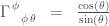

$\displaystyle \begin{array}{lcl} \Gamma_{ \phantom{\, {\phi} } \, {\phi} \, {\theta} }^{ \, {\phi} \phantom{\, {\phi} } \phantom{\, {\theta} } } & = & \frac{\cos\left({\theta}\right)}{\sin\left({\theta}\right)} \end{array}$

print(latex(nab.display(emercator)))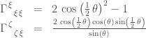

$\displaystyle \begin{array}{lcl} \Gamma_{ \phantom{\, {\xi} } \, {\xi} \, {\xi} }^{ \, {\xi} \phantom{\, {\xi} } \phantom{\, {\xi} } } & = & 2 \, \cos\left(\frac{1}{2} \, {\theta}\right)^{2} - 1 \\ \Gamma_{ \phantom{\, {\zeta} } \, {\zeta} \, {\xi} }^{ \, {\zeta} \phantom{\, {\zeta} } \phantom{\, {\xi} } } & = & \frac{2 \, \cos\left(\frac{1}{2} \, {\theta}\right) \cos\left({\theta}\right) \sin\left(\frac{1}{2} \, {\theta}\right)}{\sin\left({\theta}\right)} \end{array}$

This connection also respects the metric $g$ .

print(latex(nab(g).display()))

$\displaystyle \nabla g = 0$

Thus, since the Levi-Civita connection is unique, it must have torsion.

print(latex(nab.torsion().display(e)))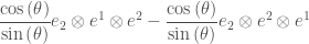

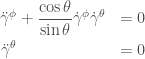
$\displaystyle \frac{\cos\left({\theta}\right)}{\sin\left({\theta}\right)} e_2\otimes e^1\otimes e^2 -\frac{\cos\left({\theta}\right)}{\sin\left({\theta}\right)} e_2\otimes e^2\otimes e^1$

The equations for geodesics are

$\displaystyle \ddot{\gamma}^k + \Gamma_{ \phantom{\, {k} } \, {i} \, {j} }^{ \, {k} \phantom{\, {i} } \phantom{\, {j} } }\dot{\gamma}^i\dot{\gamma}^j = 0$

Explicitly for both variables in the polar co-ordinates chart.

$\displaystyle \begin{aligned} \ddot{\gamma}^\phi & + \frac{\cos\theta}{\sin\theta}\dot{\gamma}^\phi\dot{\gamma}^\theta &= 0 \\ \ddot{\gamma}^\theta & &= 0 \end{aligned}$

We can check that $\gamma^\phi(t) = \alpha\log\tan t/2$ and $\gamma^\theta(t) = t$ are solutions although sage needs a bit of prompting to help it.

t = var('t'); a = var('a')

print(latex(diff(a * log(tan(t/2)),t).simplify_full()))

$\displaystyle \frac{a}{2 \, \cos\left(\frac{1}{2} \, t\right) \sin\left(\frac{1}{2} \, t\right)}$

We can simplify this further by recalling the trignometric identity.

print(latex(sin(2 * t).trig_expand()))

$\displaystyle 2 \, \cos\left(t\right) \sin\left(t\right)$

print(latex(diff (a / sin(t), t)))

$\displaystyle -\frac{a \cos\left(t\right)}{\sin\left(t\right)^{2}}$

In the mercator co-ordinates chart this is

$\displaystyle \begin{aligned} \gamma^\xi(t) &= \alpha\log\tan t/2 \\ \gamma^\zeta(t) &= \log\tan t/2 \end{aligned}$

In other words: straight lines.

Reparametersing with 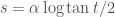$s = \alpha\log\tan t/2$ we obtain

$\displaystyle \begin{aligned} \gamma^\phi(s) &= s \\ \gamma^\theta(s) &= 2\arctan e^\frac{s}{\alpha} \end{aligned}$

Let us draw such a curve.

R.<t> = RealLine() ; print(R)

Real number line R

print(dim(R))

c = S2.curve({polar: [2*atan(exp(-t/10)), t]}, (t, -oo, +oo), name='c')

print(latex(c.display()))

$\displaystyle \begin{array}{llcl} c:& \mathbb{R} & \longrightarrow & \mathbb{S}^2 \\ & t & \longmapsto & \left({\theta}, {\phi}\right) = \left(2 \, \arctan\left(e^{\left(-\frac{1}{10} \, t\right)}\right), t\right) \\ & t & \longmapsto & \left({\xi}, {\zeta}\right) = \left(-\frac{1}{10} \, t, t\right) \end{array}$

c.parent()

$\displaystyle \mathrm{Hom}\left(\mathbb{R},\mathbb{S}^2\right)$

c.plot(chart=polar, aspect_ratio=0.1)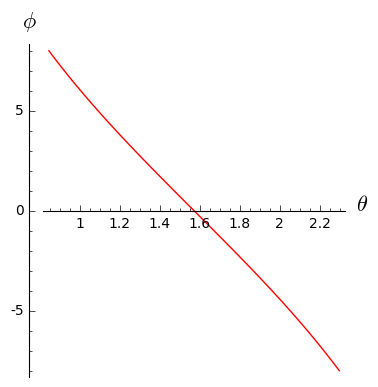

png

It’s not totally clear this is curved so let’s try with another example.

d = S2.curve({polar: [2*atan(exp(-t)), t]}, (t, -oo, +oo), name='d')

print(latex(d.display()))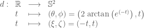

$\displaystyle \begin{array}{llcl} d:& \mathbb{R} & \longrightarrow & \mathbb{S}^2 \\ & t & \longmapsto & \left({\theta}, {\phi}\right) = \left(2 \, \arctan\left(e^{\left(-t\right)}\right), t\right) \\ & t & \longmapsto & \left({\xi}, {\zeta}\right) = \left(-t, t\right) \end{array}$

d.plot(chart=polar, aspect_ratio=0.2)

png

Now it’s clear that a straight line is curved in polar co-ordinates.

But of course in Mercator co-ordinates, it is a straight line. This explains its popularity with mariners: if you draw a straight line on your chart and follow that bearing or rhumb line using a compass you will arrive at the end of the straight line. Of course, it is not the shortest path; great circles are but is much easier to navigate.

c.plot(chart=mercator, aspect_ratio=0.1)

png

d.plot(chart=mercator, aspect_ratio=1.0)

png

We can draw these curves on the sphere itself not just on its charts.

R3 = Manifold(3, 'R^3', r'\mathbb{R}^3', start_index=1)

cart.<X,Y,Z> = R3.chart(); print(latex(cart))

$\displaystyle \left(\mathbb{R}^3,(X, Y, Z)\right)$

Phi = S2.diff_map(R3, {
    (polar, cart): [sin(th) * cos(ph), sin(th) * sin(ph), cos(th)],
    (mercator, cart): [cos(ze) / cosh(xi), sin(ze) / cosh(xi),
                       sinh(xi) / cosh(xi)]
},
    name='Phi', latex_name=r'\Phi')

We can either plot using polar co-ordinates.

graph_polar = polar.plot(chart=cart, mapping=Phi, nb_values=25, color='blue')

show(graph_polar, viewer=viewer3D)

png

Or using Mercator co-ordinates. In either case we get the sphere (minus the prime meridian).

graph_mercator = mercator.plot(chart=cart, mapping=Phi, nb_values=25, color='red')

show(graph_mercator, viewer=viewer3D)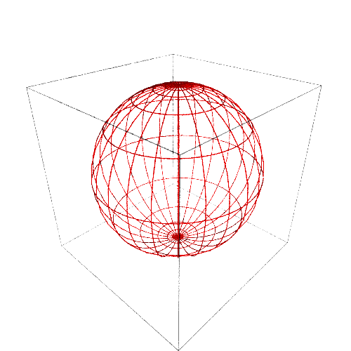

png

We can plot the curve with an angle to the meridian of $\pi/2 - \arctan 1/10$

graph_c = c.plot(mapping=Phi, max_range=40, plot_points=200, thickness=2)

show(graph_polar + graph_c, viewer=viewer3D)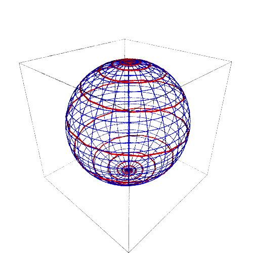

png

And we can plot the curve at angle of $\pi/4$ to the meridian.

graph_d = d.plot(mapping=Phi, max_range=40, plot_points=200, thickness=2, color="green")

show(graph_polar + graph_c + graph_d, viewer=viewer3D)

png

Haskell

With automatic differentiation and symbolic numbers, symbolic differentiation is straigtforward in Haskell.

> import Data.Number.Symbolic
> import Numeric.AD
> 
> x = var "x"
> y = var "y"
> 
> test xs = jacobian ((\x -> [x]) . f) xs
>   where
>     f [x, y] = sqrt $ x^2 + y^2

ghci> test [1, 1]
  [[0.7071067811865475,0.7071067811865475]]

ghci> test [x, y]
  [[x/(2.0*sqrt (x*x+y*y))+x/(2.0*sqrt (x*x+y*y)),y/(2.0*sqrt (x*x+y*y))+y/(2.0*sqrt (x*x+y*y))]]

Anyone wishing to take on the task of producing a Haskell version of sagemanifolds is advised to look here before embarking on the task.

Appendix A: Conformal Equivalence

Agricola and Thier (2004) shows that the geodesics of the Levi-Civita connection of a conformally equivalent metric are the geodesics of a connection with vectorial torsion. Let’s put some but not all the flesh on the bones.

The Koszul formula (see e.g. (O’Neill 1983)) characterizes the Levi-Civita connection $\nabla$

$\displaystyle \begin{aligned} 2 \langle \nabla_X Y, Z\rangle & = X \langle Y,Z\rangle + Y \langle Z,X\rangle - Z \langle X,Y\rangle \\ &- \langle X,[Y,Z]\rangle + \langle Y,[Z,X]\rangle + \langle Z,[X,Y]\rangle \end{aligned}$

Being more explicit about the metric, this can be re-written as

$\displaystyle \begin{aligned} 2 g(\nabla^g_X Y, Z) & = X g(Y,Z) + Y g(Z,X) - Z g(X,Y) \\ &- g(X,[Y,Z]) + g(Y,[Z,X]) + g(Z,[X,Y]) \end{aligned}$

Let $\nabla^h$ be the Levi-Civita connection for the metric $h = e^{2\sigma}g$ where $\sigma \in C^\infty M$ . Following [Gadea2010] and substituting into the Koszul formula and then applying the product rule

$\displaystyle \begin{aligned} 2 e^{2 \sigma} g(\nabla^h_X Y, Z) & = X e^{2 \sigma} g(Y,Z) + Y e^{2 \sigma} g(Z,X) - Z e^{2 \sigma} g(X,Y) \\ & + e^{2 \sigma} g([X,Y],Z]) - e^{2 \sigma} g([Y,Z],X) + e^{2 \sigma} g([Z,X],Y) \\ & = 2 e^{2\sigma}[g(\nabla^{g}_X Y, Z) + X\sigma g(Y,Z) + Y\sigma g(Z,X) - Z\sigma g(X,Y)] \\ & = 2 e^{2\sigma}[g(\nabla^{g}_X Y + X\sigma Y + Y\sigma X - g(X,Y) \mathrm{grad}\sigma, Z)] \end{aligned}$

Where as usual the vector field, $\mathrm{grad}\phi$ for $\phi \in C^\infty M$ , is defined via $g(\mathrm{grad}\phi, X) = \mathrm{d}\phi(X) = X\phi$ .

Let’s try an example.

nab_tilde = S2.affine_connection('nabla_t', r'\tilde_{\nabla}')

f = S2.scalar_field(-ln(sin(th)), name='f')

for i in S2.irange():
    for j in S2.irange():
        for k in S2.irange():
            nab_tilde.add_coef()[k,i,j] = \
                nab_g(polar.frame()[i])(polar.frame()[j])(polar.coframe()[k]) + \
                polar.frame()[i](f) * polar.frame()[j](polar.coframe()[k]) + \
                polar.frame()[j](f) * polar.frame()[i](polar.coframe()[k]) + \
                g(polar.frame()[i], polar.frame()[j]) * \
                polar.frame()[1](polar.coframe()[k]) * cos(th) / sin(th)

print(latex(nab_tilde.display()))

$\displaystyle \begin{array}{lcl} \Gamma_{ \phantom{\, {\theta} } \, {\theta} \, {\theta} }^{ \, {\theta} \phantom{\, {\theta} } \phantom{\, {\theta} } } & = & -\frac{\cos\left({\theta}\right)}{\sin\left({\theta}\right)} \end{array}$

print(latex(nab_tilde.torsion().display()))

g_tilde = exp(2 * f) * g

print(latex(g_tilde.parent()))

$\displaystyle \mathcal{T}^{(0,2)}\left(\mathbb{S}^2\right)$

print(latex(g_tilde[:]))

$\displaystyle \left(\begin{array}{rr} \frac{1}{\sin\left({\theta}\right)^{2}} & 0 \\ 0 & 1 \end{array}\right)$

nab_g_tilde = g_tilde.connection()

print(latex(nab_g_tilde.display()))

It’s not clear (to me at any rate) what the solutions are to the geodesic equations despite the guarantees of Agricola and Thier (2004). But let’s try a different chart.

print(latex(nab_g_tilde[emercator,:]))

$\displaystyle \left[\left[\left[0, 0\right], \left[0, 0\right]\right], \left[\left[0, 0\right], \left[0, 0\right]\right]\right]$

In this chart, the geodesics are clearly straight lines as we would hope.

References

Agricola, Ilka, and Christian Thier. 2004. “The geodesics of metric connections with vectorial torsion.” Annals of Global Analysis and Geometry 26 (4): 321–32. doi:10.1023/B:AGAG.0000047509.63818.4f.

Nakahara, M. 2003. “Geometry, Topology and Physics.” Text 822: 173–204. doi:10.1007/978-3-642-14700-5.

O’Neill, B. 1983. Semi-Riemannian Geometry with Applications to Relativity, 103. Pure and Applied Mathematics. Elsevier Science. https://books.google.com.au/books?id=CGk1eRSjFIIC.

3 thoughts on “Mercator: A Connection with Torsion”

Dominic Steinitz

November 24, 2016 at 5:08 pm

It seems my observations on cartography have been lost – sigh. I will try to reconstruct them but not today.

benmoran

December 3, 2016 at 9:40 am

Hi Dominic, great post! Is the Mercator.ipynb file available for download on Github or somewhere?

- Dominic Steinitz
  
  December 3, 2016 at 4:53 pm
  
  Glad you enjoyed it 🙂 I put it here: https://github.com/idontgetoutmuch/DifferentialGeometry but be warned you may need to install a *lot* of stuff. At least sage manifolds. If you want to draw the maps then you will need cartopy. If you want to try the Haskell then clearly Haskell and the requisite libraries. Good luck – let me know how you get on and if I can help. Also you will probably want to remove the print(latex(…)) wrapping. I put that in to generate the LaTeX for the blog post. I couldn’t get IHaskell to work so the Haskell snippet was added by hand.

Maths, Stats & Functional Programming

Formerly known as Idontgetoutmuch's Weblog

Mercator: A Connection with Torsion

Introduction

A Cartographic Aside

Colophon

Warming Up With SageManifolds

The Sphere

A New Connection

Haskell

Appendix A: Conformal Equivalence

References

3 thoughts on “Mercator: A Connection with Torsion”

Leave a comment Cancel reply

Introduction

A Cartographic Aside

Colophon

Warming Up With SageManifolds

The Sphere

A New Connection

Haskell

Appendix A: Conformal Equivalence

References

Share this:

Related

3 thoughts on “Mercator: A Connection with Torsion”

Leave a comment Cancel reply