Introduction
I was intrigued by a tweet by the UK Chancellor of the Exchequer stating "exports [to South Korea] have doubled over the last year. Now worth nearly £11bn” and a tweet by a Member of the UK Parliament stating South Korea "our second fastest growing trading partner". Although I have never paid much attention to trade statistics, both these statements seemed surprising. But these days it’s easy enough to verify such statements. It’s also an opportunity to use the techniques I believe data scientists in (computer) game companies use to determine how much impact a new feature has on the game’s consumers.
One has to be slightly careful with trade statistics as they come in many different forms, e.g., just goods or goods and services etc. When I provide software and analyses to US organisations, I am included in the services exports from the UK to the US.
Let’s analyse goods first before moving on to goods and services.
Getting the Data
First let’s get hold of the quarterly data from the UK Office of National Statistics.
ukstats <- "https://www.ons.gov.uk"
bop <- "economy/nationalaccounts/balanceofpayments"
ds <- "datasets/tradeingoodsmretsallbopeu2013timeseriesspreadsheet/current/mret.csv"

mycsv <- read.csv(paste(ukstats,"file?uri=",bop,ds,sep="/"),stringsAsFactors=FALSE)
Now we can find the columns that refer to Korea.
ns <- which(grepl("Korea", names(mycsv)))
length(ns)
## [1] 3names(mycsv[ns[1]])## [1] "BoP.consistent..South.Korea..Exports..SA................................"names(mycsv[ns[2]])## [1] "BoP.consistent..South.Korea..Imports..SA................................"names(mycsv[ns[3]])## [1] "BoP.consistent..South.Korea..Balance..SA................................"Now we can pull out the relevant information and create a data frame of it.
korean <- mycsv[grepl("Korea", names(mycsv))]
imports <- korean[grepl("Imports", names(korean))]
exports <- korean[grepl("Exports", names(korean))]
balance <- korean[grepl("Balance", names(korean))]

df <- data.frame(mycsv[grepl("Title", names(mycsv))],
                 imports,
                 exports,
                 balance)
colnames(df) <- c("Title", "Imports", "Exports", "Balance")

startQ <- which(grepl("1998 Q1",df$Title))
endQ <- which(grepl("2016 Q3",df$Title))
dfQ <- df[startQ:endQ,]
We can now plot the data.
tab <- data.frame(kr=as.numeric(dfQ$Exports),
                  krLabs=as.numeric(as.Date(as.yearqtr(dfQ$Title,format='%Y Q%q'))))

ggplot(tab, aes(x=as.Date(tab$krLabs), y=tab$kr)) + geom_line() +
    theme(legend.position="bottom") +
    ggtitle("Goods Exports UK / South Korea (Quarterly)") +
    theme(plot.title = element_text(hjust = 0.5)) +
    xlab("Date") +
    ylab("Value (£m)")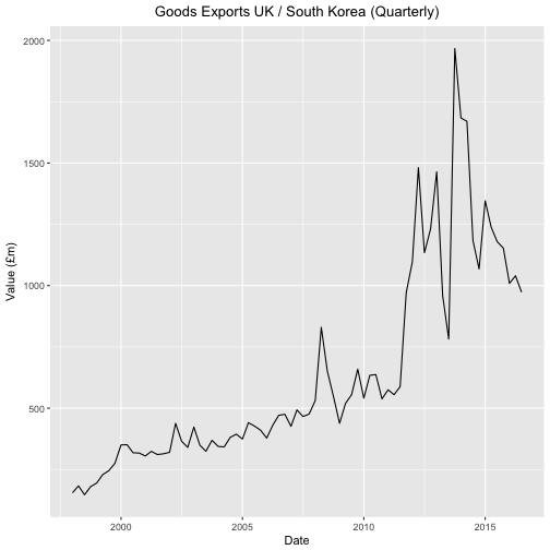
For good measure let’s plot the annual data.
startY <- grep("^1998$",df$Title)
endY <- grep("^2015$",df$Title)
dfYear <- df[startY:endY,]

tabY <- data.frame(kr=as.numeric(dfYear$Exports),
                   krLabs=as.numeric(dfYear$Title))

ggplot(tabY, aes(x=tabY$krLabs, y=tabY$kr)) + geom_line() +
    theme(legend.position="bottom") +
    ggtitle("Goods Exports UK / South Korea (Annual)") +
    theme(plot.title = element_text(hjust = 0.5)) +
    xlab("Date") +
    ylab("Value (£m)")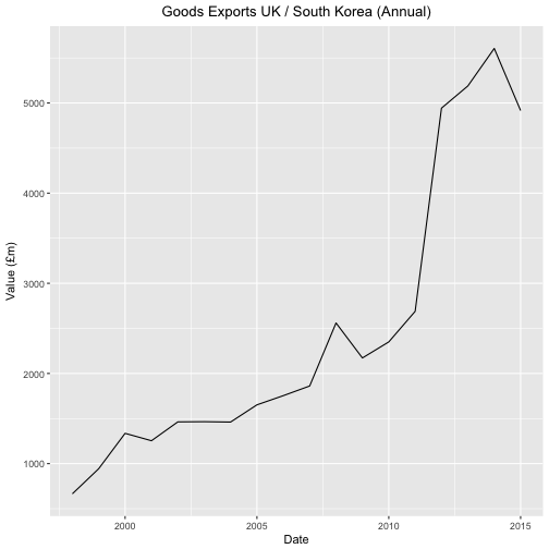
And the monthly data.
startM <- grep("1998 JAN",df$Title)
endM <- grep("2016 OCT",df$Title)
dfMonth <- df[startM:endM,]

tabM <- data.frame(kr=as.numeric(dfMonth$Exports),
                   krLabs=as.numeric(as.Date(as.yearmon(dfMonth$Title,format='%Y %B'))))

ggplot(tabM, aes(x=as.Date(tabM$krLabs), y=tabM$kr)) + geom_line() +
    theme(legend.position="bottom") +
    ggtitle("Goods Exports UK / South Korea (Monthly)") +
    theme(plot.title = element_text(hjust = 0.5)) +
    xlab("Date") +
    ylab("Value (£m)")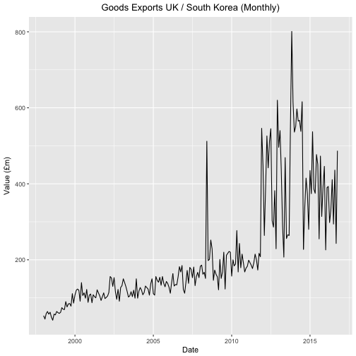
It looks like some change took place in 2011 but nothing to suggest either that "export have doubled over the last year" or that South Korea is "our second fastest growing partner". That some sort of change did happen is further supported by the fact a Free Trade Agreement between the EU and Korea was put in place in 2011.
But was there really a change? And what sort of change was it? Sometimes it’s easy to imagine patterns where there are none.

With this warning in mind let us see if we can get a better feel from the numbers as to what happened.
The Model
Let us assume that the data for exports are approximated by a linear function of time but that there is a change in the slope and the offset at some point during observation.
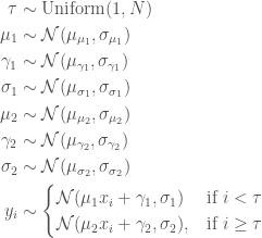
Since we are going to use stan to infer the parameters for this model and stan cannot handle discrete parameters, we need to marginalize out this (discrete) parameter. I hope to do the same analysis with LibBi which seems more suited to time series analysis and which I believe will not require such a step.
Setting D = {yi}i = 1N we can calculate the likelihood
stan operates on the log scale and thus requires the log likelihood
where
and where the log sum of exponents function is defined by

The log sum of exponents function allows the model to be coded directly in Stan using the built-in function , which provides both arithmetic stability and efficiency for mixture model calculations.
Stan
Here’s the model in stan. Sadly I haven’t found a good way of divvying up .stan files in a .Rmd file so that it still compiles.
data {
  int<lower=1> N;
  real x[N];
  real y[N];
}

parameters {
  real mu1;
  real mu2;
  real gamma1;
  real gamma2;

  real<lower=0> sigma1;
  real<lower=0> sigma2;
}

transformed parameters {
      vector[N] log_p;
      real mu;
      real sigma;
      log_p = rep_vector(-log(N), N);
      for (tau in 1:N)
        for (i in 1:N) {
          mu = i < tau ? (mu1 * x[i] + gamma1) : (mu2 * x[i] + gamma2);
          sigma = i < tau ? sigma1 : sigma2;
          log_p[tau] = log_p[tau] + normal_lpdf(y[i] | mu, sigma);
      }
}

model {
    mu1 ~ normal(0, 10);
    mu2 ~ normal(0, 10);
    gamma1 ~ normal(0, 10);
    gamma2 ~ normal(0, 10);
    sigma1 ~ normal(0, 10);
    sigma2 ~ normal(0, 10);

    target += log_sum_exp(log_p);
}

generated quantities {
    int<lower=1,upper=N> tau;
    tau = categorical_rng(softmax(log_p));
}
The above, although mimicking our mathematical model, has quadratic complexity and we can use the trick in the stan manual to make it linear albeit with less clarity.
data {
  int<lower=1> N;
  real x[N];
  real y[N];
}

parameters {
  real mu1;
  real mu2;
  real gamma1;
  real gamma2;

  real<lower=0> sigma1;
  real<lower=0> sigma2;
}

transformed parameters {
  vector[N] log_p;
  {
    vector[N+1] log_p_e;
    vector[N+1] log_p_l;
    log_p_e[1] = 0;
    log_p_l[1] = 0;
    for (i in 1:N) {
      log_p_e[i + 1] = log_p_e[i] + normal_lpdf(y[i] | mu1 * x[i] + gamma1, sigma1);
      log_p_l[i + 1] = log_p_l[i] + normal_lpdf(y[i] | mu2 * x[i] + gamma2, sigma2);
    }
    log_p = rep_vector(-log(N) + log_p_l[N + 1], N) + head(log_p_e, N) - head(log_p_l, N);
  }
}

model {
    mu1 ~ normal(0, 10);
    mu2 ~ normal(0, 10);
    gamma1 ~ normal(0, 10);
    gamma2 ~ normal(0, 10);
    sigma1 ~ normal(0, 10);
    sigma2 ~ normal(0, 10);

    target += log_sum_exp(log_p);
}

generated quantities {
    int<lower=1,upper=N> tau;
    tau = categorical_rng(softmax(log_p));
}
Let’s run this model with the monthly data.
NM <- nrow(tabM)
KM <- ncol(tabM)

yM <- tabM$kr
XM <- data.frame(tabM,rep(1,NM))[,2:3]

fitM <- stan(
    file = "lr-changepoint-ng.stan",
    data = list(x = XM$krLabs, y = yM, N = length(yM)),
    chains = 4,
    warmup = 1000,
    iter = 10000,
    cores = 4,
    refresh = 500,
    seed=42
)
## Warning: There were 662 divergent transitions after warmup. Increasing adapt_delta above 0.8 may help. See
## http://mc-stan.org/misc/warnings.html#divergent-transitions-after-warmup## Warning: Examine the pairs() plot to diagnose sampling problemsLooking at the results below we see a multi-modal distribution so a mean is not of much use.
histData <- hist(extract(fitM)$tau,plot=FALSE,breaks=c(seq(1,length(yM),1)))
histData$counts
## [1] 18000 0 0 0 0 0 0 0 0 0 0
## [12] 0 0 0 0 0 0 0 0 0 0 0
## [23] 0 0 0 0 0 0 0 0 0 0 0
## [34] 0 0 0 0 0 0 0 0 0 0 0
## [45] 0 0 0 0 0 0 0 0 0 0 0
## [56] 0 0 0 0 0 0 0 0 0 0 0
## [67] 0 0 0 0 0 0 0 0 0 0 0
## [78] 0 0 0 0 0 0 0 0 0 0 0
## [89] 0 0 0 0 0 0 0 0 0 0 0
## [100] 0 0 0 0 0 0 0 0 0 0 0
## [111] 0 0 0 0 0 0 0 1 4 12 16
## [122] 16 107 712 8132 0 0 0 0 0 0 0
## [133] 0 0 0 0 0 0 0 0 0 0 0
## [144] 0 0 0 0 0 0 0 0 0 0 0
## [155] 0 0 0 0 0 0 0 0 0 0 25
## [166] 171 2812 0 0 0 0 0 0 0 0 0
## [177] 0 0 0 0 0 0 0 0 0 0 0
## [188] 0 0 0 0 0 0 0 0 0 0 0
## [199] 0 0 0 0 0 0 0 0 0 0 0
## [210] 0 0 0 0 0 0 0 0 0 0 0
## [221] 0 0 0 0 5992We can get a pictorial representation of the maxima so that the multi-modality is even clearer.
min_indexes = which(diff(  sign(diff( c(0,histData$counts,0)))) == 2)
max_indexes = which(diff(  sign(diff( c(0,histData$counts,0)))) == -2)
modeData = data.frame(x=1:length(histData$counts),y=histData$counts)
min_locs = modeData[min_indexes,]
max_locs = modeData[max_indexes,]
plot(modeData$y, type="l")
points( min_locs, col="red", pch=19, cex=1  )
points( max_locs, col="green", pch=19, cex=1  )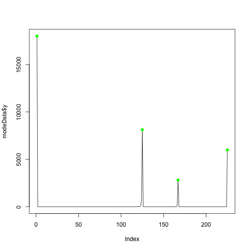
My interpretation is that the evidence (data) says there is probably no changepoint (a change at the beginning or end is no change) but there might be a change at intermediate data points.
We can see something strange (maybe a large single export?) happened at index 125 which translates to 2008MAY.
The mode at index 167 which translates to 2011NOV corresponds roughly to the EU / Korea trade agreement.
Let us assume that there really was a material difference in trade at this latter point. We can fit a linear regression before this point and one after this point.
Here’s the stan
data {
  int<lower=1> N;
  int<lower=1> K;
  matrix[N,K]  X;
  vector[N]    y;
}
parameters {
  vector[K] beta;
  real<lower=0> sigma;
}
model {
  y ~ normal(X * beta, sigma);
}
And here’s the R to fit the before and after data. We fit the model, pull out the parameters for the regression and pull out the covariates
N <- length(yM)
M <- max_locs$x[3]

fite <- stan(file = 'LR.stan',
             data = list(N = M, K = ncol(XM), y = yM[1:M], X = XM[1:M,]),
             pars=c("beta", "sigma"),
             chains=3,
             cores=3,
             iter=3000,
             warmup=1000,
             refresh=-1)

se <- extract(fite, pars = c("beta", "sigma"), permuted=TRUE)
estCovParamsE <- colMeans(se$beta)

fitl <- stan(file = 'LR.stan',
             data = list(N = N-M, K = ncol(XM), y = yM[(M+1):N], X = XM[(M+1):N,]),
             pars=c("beta", "sigma"),
             chains=3,
             cores=3,
             iter=3000,
             warmup=1000,
             refresh=-1)

sl <- extract(fitl, pars = c("beta", "sigma"), permuted=TRUE)
estCovParamsL <- colMeans(sl$beta)
Make predictions
linRegPredsE <- data.matrix(XM) %*% estCovParamsE
linRegPredsL <- data.matrix(XM) %*% estCovParamsLggplot(tabM, aes(x=as.Date(tabM$krLabs), y=tabM$kr)) +
geom_line(aes(x = as.Date(tabM$krLabs), y = tabM$kr, col = "Actual")) +
geom_line(data=tabM[1:M,], aes(x = as.Date(tabM$krLabs[1:M]), y = linRegPredsE[(1:M),1], col = "Fit (Before FTA)")) +
geom_line(data=tabM[(M+1):N,], aes(x = as.Date(tabM$krLabs[(M+1):N]), y = linRegPredsL[((M+1):N),1], col = "Fit (After FTA)")) +
theme(legend.position="bottom") +
ggtitle("Goods Exports UK / South Korea (Monthly)") +
theme(plot.title = element_text(hjust = 0.5)) +
xlab("Date") +
ylab("Value (£m)")
An Intermediate Conclusion and Goods and Services (Pink Book)
So we didn’t manage to substantiate either the Chancellor’s claim or the Member of Parliament’s claim.
But it may be that we can if we look at Goods and Services then we might be able to see the numbers resulting in the claims.
pb <- "datasets/pinkbook/current/pb.csv"
pbcsv <- read.csv(paste(ukstats,"file?uri=",bop,pb,sep="/"),stringsAsFactors=FALSE)
This has a lot more information albeit only annually.
pbns <- grep("Korea", names(pbcsv))
length(pbns)
## [1] 21lapply(pbns,function(x) names(pbcsv[x]))## [[1]]
## [1] "BoP..Current.Account..Goods...Services..Imports..South.Korea............"
##
## [[2]]
## [1] "BoP..Current.Account..Current.Transfer..Balance..South.Korea............"
##
## [[3]]
## [1] "BoP..Current.Account..Goods...Services..Balance..South.Korea............"
##
## [[4]]
## [1] "IIP..Assets..Total.South.Korea.........................................."
##
## [[5]]
## [1] "Trade.in.Services.replaces.1.A.B....Exports.Credits...South.Korea...nsa."
##
## [[6]]
## [1] "IIP...Liabilities...Total...South.Korea................................."
##
## [[7]]
## [1] "BoP..Total.income..Balance..South.Korea................................."
##
## [[8]]
## [1] "BoP..Total.income..Debits..South.Korea.................................."
##
## [[9]]
## [1] "BoP..Total.income..Credits..South.Korea................................."
##
## [[10]]
## [1] "BoP..Current.account..Balance..South.Korea.............................."
##
## [[11]]
## [1] "BoP..Current.account..Debits..South.Korea..............................."
##
## [[12]]
## [1] "BoP..Current.account..Credits..South.Korea.............................."
##
## [[13]]
## [1] "IIP...Net...Total....South.Korea........................................"
##
## [[14]]
## [1] "Trade.in.Services.replaces.1.A.B....Imports.Debits...South.Korea...nsa.."
##
## [[15]]
## [1] "BoP..Current.Account..Services..Total.Balance..South.Korea.............."
##
## [[16]]
## [1] "Bop.consistent..Balance..NSA..South.Korea..............................."
##
## [[17]]
## [1] "Bop.consistent..Im..NSA..South.Korea...................................."
##
## [[18]]
## [1] "Bop.consistent..Ex..NSA..South.Korea...................................."
##
## [[19]]
## [1] "Current.Transfers...Exports.Credits...South.Korea...nsa................."
##
## [[20]]
## [1] "Current.Transfers...Imports.Debits...South.Korea...nsa.................."
##
## [[21]]
## [1] "BoP..Current.Account..Goods...Services..Exports..South.Korea............"Let’s just look at exports.
koreanpb <- pbcsv[grepl("Korea", names(pbcsv))]
exportspb <- koreanpb[grepl("Exports", names(koreanpb))]
names(exportspb)
## [1] "Trade.in.Services.replaces.1.A.B....Exports.Credits...South.Korea...nsa."
## [2] "Current.Transfers...Exports.Credits...South.Korea...nsa................."
## [3] "BoP..Current.Account..Goods...Services..Exports..South.Korea............"The last column gives exports of Goods and Services so let’s draw a chart of it.
pb <- data.frame(pbcsv[grepl("Title", names(pbcsv))],
                 exportspb[3])
colnames(pb) <- c("Title", "Exports")

startpbY <- which(grepl("1999",pb$Title))
endpbY <- which(grepl("2015",pb$Title))
pbY <- pb[startpbY:endpbY,]

tabpbY <- data.frame(kr=as.numeric(pbY$Exports),
                     krLabs=as.numeric(pbY$Title))

ggplot(tabpbY, aes(x=tabpbY$krLabs, y=tabpbY$kr)) + geom_line() +
    theme(legend.position="bottom") +
    ggtitle("Goods and Services Exports UK / South Korea (Annual)") +
    theme(plot.title = element_text(hjust = 0.5)) +
    xlab("Date") +
    ylab("Value (£m)")
No joy here either to any of the claims. Still it’s been an interesting exercise.

Well done your excellent work is confirmed by the UKGOV
the European Union (EU)-Korea Free Trade Agreement (FTA), the only EU FTA in east Asia/Pacific, is estimated to be worth over £500 million to UK business each year https://www.gov.uk/government/publications/exporting-to-south-korea/exporting-to-south-korea
i hope you do not mind I referenced your work on my page
I am glad you found it useful.
It is an excellent and well-presented work. If I ever become a multi-billionaire with a Global Empire employing thousands of people I will make you the head of my Audit Group.
As a data scientists in a (computer) game company I approve of this analysis! 🙂
Without haven given it too much though: Is it really necessary to model the change point parameter tau as discrete? I’m thinking that it could be ok to model it as continuous, which would make everything easier in STAN, even if it’s not strictly correct?
I like it 🙂 – I will try when I have time