Introduction

We previously used importance sampling in the case where we did not have a sampler available for the distribution from which we wished to sample. There is an even more compelling case for using importance sampling.

Suppose we wish to estimate the probability of a rare event. For example, suppose we wish to estimate $\mathbb{P}(X > 5)$ where $X \sim {\mathcal{N}}(0,1)$ . In this case, we can look up the answer $\mathbb{P}(X > 5) \approx 2.86710^{-7}$ . But suppose we couldn’t look up the answer. One strategy that might occur to us is to sample and then estimate the probability by counting the number of times out of the total that the sample was bigger than 5. The flaw in this is obvious but let’s try it anyway.

> module Girsanov where

> import qualified Data.Vector as V
> import Data.Random.Source.PureMT
> import Data.Random
> import Control.Monad.State
> import Data.Histogram.Fill
> import Data.Histogram.Generic ( Histogram )
> import Data.Number.Erf
> import Data.List ( transpose )

> samples :: (Foldable f, MonadRandom m) =>
>                     (Int -> RVar Double -> RVar (f Double)) ->
>                     Int ->
>                     m (f Double)
> samples repM n = sample $ repM n $ stdNormal

> biggerThan5 :: Int
> biggerThan5 = length (evalState xs (pureMT 42))
>   where
>     xs :: MonadRandom m => m [Double]
>     xs = liftM (filter (>= 5.0)) $ samples replicateM 100000

As we might have expected, even if we draw 100,000 samples, we estimate this probability quite poorly.

ghci> biggerThan5
  0

Using importance sampling we can do a lot better.

Let $\xi$ be a normally distributed random variable with zero mean and unit variance under the Lebesgue measure $\mathbb{P}$ . As usual we can then define a new probability measure, the law of $\xi$ , by

$\displaystyle \begin{aligned} \mathbb{P}_\xi((-\infty, b]) &= \frac{1}{\sqrt{2\pi}}\int_{-\infty}^b e^{-x^2/2}\,\mathrm{d}x \end{aligned}$

Thus

$\displaystyle \begin{aligned} \mathbb{E}_\xi(f) &= \frac{1}{\sqrt{2\pi}}\int_{-\infty}^\infty f(x) e^{-x^2/2}\,\mathrm{d}x \\ &= \frac{1}{\sqrt{2\pi}}\int_{-\infty}^\infty f(x) e^{a^2/2}e^{-a x}e^{-(x-a)^2/2}\,\mathrm{d}x \\ &= \mathbb{E}_{\xi + a}(fg) \\ &= \mathbb{\tilde{E}}_{\xi + a}(f) \end{aligned}$

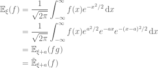
where we have defined

$\displaystyle g(x) \triangleq e^{a^2/2}e^{-a x} \quad \mathrm{and} \quad \mathbb{\tilde{P}}((-\infty, b]) \triangleq \int_{-\infty}^b g(x)\,\mathrm{d}x$

Thus we can estimate $\mathbb{P}(X > 5)$ either by sampling from a normal distribution with mean 0 and counting the number of samples that are above 5 or we can sample from a normal distribution with mean 5 and calculating the appropriately weighted mean

$\displaystyle \frac{1}{n}\sum_{i=1}^n \mathbb{I}_{\{x > 5\}}g(y)$

Let’s try this out.

> biggerThan5' :: Double
> biggerThan5' = sum (evalState xs (pureMT 42)) / (fromIntegral n)
>   where
>     xs :: MonadRandom m => m [Double]
>     xs = liftM (map g) $
>          liftM (filter (>= 5.0)) $
>          liftM (map (+5)) $
>          samples replicateM n
>     g x = exp $ (5^2 / 2) - 5 * x
>     n = 100000

And now we get quite a good estimate.

ghci> biggerThan5'
  2.85776225450217e-7

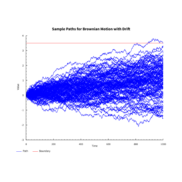
Random Paths

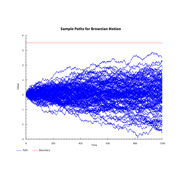
The probability of another rare event we might wish to estimate is that of Brownian Motion crossing a boundary. For example, what is the probability of Browian Motion crossing the line $y = 3.5$ ? Let’s try sampling 100 paths (we restrict the number so the chart is still readable).

> epsilons :: (Foldable f, MonadRandom m) =>
>                     (Int -> RVar Double -> RVar (f Double)) ->
>                     Double ->
>                     Int ->
>                     m (f Double)
> epsilons repM deltaT n = sample $ repM n $ rvar (Normal 0.0 (sqrt deltaT))

> bM0to1 :: Foldable f =>
>           ((Double -> Double -> Double) -> Double -> f Double -> f Double)
>           -> (Int -> RVar Double -> RVar (f Double))
>           -> Int
>           -> Int
>           -> f Double
> bM0to1 scan repM seed n =
>   scan (+) 0.0 $
>   evalState (epsilons repM (recip $ fromIntegral n) n) (pureMT (fromIntegral seed))

We can see by eye in the chart below that again we do quite poorly.

We know that $\mathbb{P}(T_a \leq t) = 2(1 - \Phi (a / \sqrt{t}))$ where $T_a = \inf \{t : W_t = a\}$ .

> p :: Double -> Double -> Double
> p a t = 2 * (1 - normcdf (a / sqrt t))

ghci> p 1.0 1.0
  0.31731050786291415

ghci> p 2.0 1.0
  4.550026389635842e-2

ghci> p 3.0 1.0
  2.699796063260207e-3

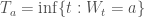
But what if we didn’t know this formula? Define

$\displaystyle N(\omega) \triangleq \begin{cases} 1 & \text{if } \sup_{0 \leq t \leq 1}\tilde W_t \geq a \\ 0 & \text{if } \sup_{0 \leq t \leq 1}\tilde W_t < a \\ \end{cases}$

where $\mathbb{Q}$ is the measure which makes $\tilde W_t$ Brownian Motion.

We can estimate the expectation of $N$

$\displaystyle \hat p_{\mathbb{Q}} = \frac{1}{M}\sum_{i=1}^H n_i$

where $n_i$ is 1 if Brownian Motion hits the barrier and 0 otherwise and M is the total number of simulations. We know from visual inspection that this gives poor results but let us try some calculations anyway.

> n = 500
> m = 10000

> supAbove :: Double -> Double
> supAbove a = fromIntegral count / fromIntegral n
>   where
>     count = length $
>             filter (>= a) $
>             map (\seed -> maximum $ bM0to1 scanl replicateM seed m) [0..n - 1]

> bM0to1WithDrift seed mu n =
>   zipWith (\m x -> x + mu * m * deltaT) [0..] $
>   bM0to1 scanl replicateM seed n
>     where
>       deltaT = recip $ fromIntegral n

ghci> supAbove 1.0
  0.326

ghci> supAbove 2.0
  7.0e-2

ghci> supAbove 3.0
  0.0

As expected for a rare event we get an estimate of 0.

Fortunately we can use importance sampling for paths. If we take $\mu(\omega, t) = a$ where $a$ is a constant in Girsanov’s Theorem below then we know that $\tilde W_t = W_t + \int_0^t a \,\mathrm{d}s = W_t + at$ is $\mathbb{Q}$ -Brownian Motion.

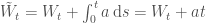
We observe that

$\displaystyle \begin{aligned} \mathbb{Q}N &= \mathbb{P}\bigg(N\frac{\mathrm{d} \mathbb{Q}}{\mathrm{d} \mathbb{P}}\bigg) \\ &= \mathbb{P}\Bigg[N \exp \Bigg(-\int_0^1 \mu(\omega,t) \,\mathrm{d}W_t - \frac{1}{2} \int_0^1 \mu^2(\omega, t) \,\mathrm{d} t\Bigg) \Bigg] \\ &= \mathbb{P}\Bigg[N \exp \Bigg(-aW_1 - \frac{1}{2} a^2\Bigg) \Bigg] \end{aligned}$

So we can also estimate the expectation of $N$ under $\mathbb{P}$ as

$\displaystyle \hat p_{\mathbb{P}} = \frac{1}{M}\sum_{i=1}^H n_i\exp{\bigg(-aw^{(1)}_i - \frac{a^2}{2}\bigg)}$

where $n_i$ is now 1 if Brownian Motion with the specified drift hits the barrier and 0 otherwise, and $w^{(1)}_i$ is Brownian Motion sampled at $t=1$ .

We can see from the chart below that this is going to be better at hitting the required barrier.

Let’s do some calculations.

> supAbove' a = (sum $ zipWith (*) ns ws) / fromIntegral n
>   where
>     deltaT = recip $ fromIntegral m
> 
>     uss = map (\seed -> bM0to1 scanl replicateM seed m) [0..n - 1]
>     ys = map last uss
>     ws = map (\x -> exp (-a * x - 0.5 * a^2)) ys
> 
>     vss = map (zipWith (\m x -> x + a * m * deltaT) [0..]) uss
>     sups = map maximum vss
>     ns = map fromIntegral $ map fromEnum $ map (>=a) sups

ghci> supAbove' 1.0
  0.31592655955519156

ghci> supAbove' 2.0
  4.999395029856741e-2

ghci> supAbove' 3.0
  2.3859203473651654e-3

The reader is invited to try the above estimates with 1,000 samples per path to see that even with this respectable number, the calculation goes awry.

In General

If we have a probability space $(\Omega, {\mathcal{F}}, \mathbb{P})$ and a non-negative random variable $Z$ with $\mathbb{E}Z = 1$ then we can define a new probability measure $\mathbb{Q}$ on the same $\sigma$ -algebra by

$\displaystyle \mathbb{Q} A \triangleq \int_A Z \,\mathrm{d} \mathbb{P}$

For any two probability measures when such a $Z$ exists, it is called the Radon-Nikodym derivative of $\mathbb{Q}$ with respect to $\mathbb{P}$ and denoted $\frac{\mathrm{d} \mathbb{Q}}{\mathrm{d} \mathbb{P}}$

Given that we managed to shift a Normal Distribution with non-zero mean in one measure to a Normal Distribution with another mean in another measure by producing the Radon-Nikodym derivative, might it be possible to shift, Brownian Motion with a drift under a one probability measure to be pure Brownian Motion under another probability measure by producing the Radon-Nikodym derivative? The answer is yes as Girsanov’s theorem below shows.

Girsanov’s Theorem

Let $W_t$ be Brownian Motion on a probability space $(\Omega, {\mathcal{F}}, \mathbb{P})$ and let $\{{\mathcal{F}}_t\}_{t \in [0,T]}$ be a filtration for this Brownian Motion and let $\mu(\omega, t)$ be an adapted process such that the Novikov Sufficiency Condition holds

$\displaystyle \mathbb{E}\bigg[\exp{\bigg(\frac{1}{2}\int_0^T \mu^2(s, \omega) \,\mathrm{d}s\bigg)}\bigg] = K < \infty$

then there exists a probability measure $\mathbb{Q}$ such that

$\mathbb{Q}$ is equivalent to $\mathbb{P}$ , that is, $\mathbb{Q}(A) = 0 \iff \mathbb{P}(A) = 0$ .
$\displaystyle {\frac{\mathrm{d}\mathbb{Q}}{\mathrm{d}\mathbb{P}} = \exp \Bigg(-\int_0^T \mu(\omega,t) \,\mathrm{d}W_t - \frac{1}{2} \int_0^T \mu^2(\omega, t) \,\mathrm{d} t\Bigg)}$ .
$\tilde W_t = W_t + \int_0^t \mu(\omega, t) \,\mathrm{d}s$ is Brownian Motion on the probabiity space $(\Omega, {\mathcal{F}}, \mathbb{Q})$ also with the filtration $\{\mathcal{F}_t\}_{t \in [0,T]}$ .

In order to prove Girsanov’s Theorem, we need a condition which allows to infer that $M_t(\mu)$ is a strict martingale. One such useful condition to which we have already alluded is the Novikov Sufficiency Condition.

Proof

Define $\mathbb{Q}$ by

$\displaystyle \mathbb{Q}(A) = \mathbb{P}(1_A M_T) \quad \mathrm{where} \quad M_t(\mu) = \exp{\bigg(\int_0^t - \mu(t, \omega) \,\mathrm{d}W_s - \frac{1}{2}\int_0^t \mu^2(t, \omega) \,\mathrm{d}s\bigg)}$

Then, temporarily overloading the notation and writing $\mathbb{P}$ for expectation under $\mathbb{P}$ , and applying the Novikov Sufficiency Condition to $f(s) - \mu(\omega ,s)$ , we have

$\displaystyle \begin{aligned} \mathbb{Q}\bigg[\exp{\int_0^T f(s) \,\mathrm{d}X_s}\bigg] &= \mathbb{Q}\bigg[\exp{\int_0^T f(s) \,\mathrm{d}W_s + \int_0^T \mu(\omega, s) \,\mathrm{d}s}\bigg] \\ &= \mathbb{P}\bigg[\exp{\bigg( \int_0^T \big(f(s) - \mu(\omega, s)\big)\,\mathrm{d}W_s + \int_0^T f(s)\mu(\omega, s)\,\mathrm{d}s - \frac{1}{2}\int_0^T \mu^2(\omega ,s) \,\mathrm{d}s \bigg)}\bigg] \\ &= \mathbb{P}\bigg[\exp{\bigg( \int_0^T \big(f(s) - \mu(\omega, s)\big)\,\mathrm{d}W_s - \frac{1}{2}\int_0^T \big(f(s) - \mu(\omega ,s)\big)^2 \,\mathrm{d}s + \frac{1}{2}\int_0^T f^2(s) \,\mathrm{d}s \bigg)}\bigg] \\ &= \frac{1}{2}\int_0^T f^2(s) \,\mathrm{d}s \, \mathbb{P}\bigg[\exp{\bigg( \int_0^T \big(f(s) - \mu(\omega, s)\big)\,\mathrm{d}W_s - \frac{1}{2}\int_0^T \big(f(s) - \mu(\omega ,s)\big)^2 \,\mathrm{d}s \bigg)}\bigg] \\ &= \frac{1}{2}\int_0^T f^2(s) \,\mathrm{d}s \end{aligned}$

From whence we see that

$\displaystyle \mathbb{Q}\big(e^{i \zeta (X_t - X_s)}\big) = e^{-\frac{1}{2} \zeta^2 (t - s)}$

And since this characterizes Brownian Motion, we are done.

$\blacksquare$

The Novikov Sufficiency Condition

The Novikov Sufficiency Condition Statement

Let $\mu \in {\cal{L}}^2_{\mathrm{LOC}}[0,T]$ and further let it satisfy the Novikov condition

$\displaystyle \mathbb{E}\bigg[\exp{\bigg(\frac{1}{2}\int_0^T \mu^2(s, \omega) \,\mathrm{d}s\bigg)}\bigg] = K < \infty$

then the process defined by

$\displaystyle M_t(\mu) = \exp{\bigg(\int_0^t \mu(t, \omega) \,\mathrm{d}W_s - \frac{1}{2}\int_0^t \mu^2(t, \omega) \,\mathrm{d}s\bigg)}$

is a strict martingale.

Before we prove this, we need two lemmas.

Lemma 1

Let $M_t$ for $t \in [0,t]$ be a non-negative local martingale then $M_t$ is a super-martingale and if further $\mathbb{E}M_T = \mathbb{E}M_0$ then $M_t$ is a strict martingale.

Proof

Let $\{\tau_n\}_{n \in \mathbb{N}}$ be a localizing sequence for $M_t$ then for $0 < s < t < T$ and using Fatou’s lemma and the fact that the stopped process is a strict martingale

$\displaystyle \mathbb{E}(M_t \,|\, {\mathcal{F}_s}) = \mathbb{E}(\liminf_{n \rightarrow \infty} M_{t \land \tau_m} \,|\, {\mathcal{F}_s}) \leq \liminf_{n \rightarrow \infty} \mathbb{E}(M_{t \land \tau_m} \,|\, {\mathcal{F}_s}) = \liminf_{n \rightarrow \infty} M_{s \land \tau_m} = M_s$

Thus $M_t$ is a super-martingale and therefore

$\displaystyle \mathbb{E}M_T \leq \mathbb{E}M_t \leq \mathbb{E}M_s \leq \mathbb{E}M_0$

By assumption we have $\mathbb{E}M_T \leq \mathbb{E}M_0$ thus $M_t$ is a strict martingale.

$\blacksquare$

Lemma 2

Let $M_t$ be a non-negative local martingale. If $\{\tau_n\}_{n \in \mathbb{N}}$ is a localizing sequence such that $\sup_n \|M_{T \land \tau_n}\|_p < \infty$ for some $p > 1$ then $M_t$ is a strict martingale.

Proof

$\displaystyle \mathbb{E}(|M_T - M_{T \land \tau_n}|) \leq \mathbb{E}(|M_T - r \land M_T) + \mathbb{E}(|r \land M_T - r \land M_{T \land \tau_n}|) + \mathbb{E}(M_{T \land \tau_n} - r \land M_{T \land \tau_n})$

By the super-martingale property $\mathbb{E}(M_T) \leq \mathbb{E}(M_0) < \infty$ and thus by dominated convergence we have that

$\displaystyle \lim_{r \rightarrow \infty} \mathbb{E}(r \land M_T) = \mathbb{E}(M_T) \quad \mathrm{and} \quad \lim_{r \rightarrow \infty}\lim_{n \rightarrow \infty}\mathbb{E}(|r \land M_T - r \land M_{T \land \tau_n}|) = 0$

We also have that

$\displaystyle \begin{aligned} \mathbb{E}(M_{T \land \tau_n} - r \land M_{T \land \tau_n}) &= \mathbb{E}((M_{T \land \tau_n} - r \land M_{T \land \tau_n}){I}_{(M_{T \land \tau_n} > r)}) + \mathbb{E}((M_{T \land \tau_n} - r \land M_{T \land \tau_n}){I}_{(M_{T \land \tau_n} \leq r)}) \\ &= \mathbb{E}((M_{T \land \tau_n} - r \land M_{T \land \tau_n}){I}_{(M_{T \land \tau_n} > r)}) \\ &= \mathbb{E}(M_{T \land \tau_n}{I}_{(M_{T \land \tau_n} > r)}) - r\mathbb{P}({M_{T \land \tau_n} > r}) \end{aligned}$

By Chebyshev’s inequality (see note (2) below), we have

$\displaystyle r\mathbb{P}({M_{T \land \tau_n} > r}) \leq \frac{r\mathbb{E}|X|^p}{r^p} \leq \frac{\sup_n{\mathbb{E}(M_{T \land \tau_n})^p}}{r^{p-1}}$

Taking limits first over $n \rightarrow \infty$ and then over $r \rightarrow \infty$ we see that

$\displaystyle \lim_{r \rightarrow \infty}\lim_{n \rightarrow \infty} r\mathbb{P}({M_{T \land \tau_n} > r}) \rightarrow 0$

For $0 \leq r \leq x$ and $p > 1$ we have $x \leq r^{1-p}x^p$ . Thus

$\displaystyle \mathbb{E}(M_{T \land \tau_n}{I}_{(M_{T \land \tau_n} > r)}) \leq r^{1-p}\mathbb{E}(M_{T \land \tau_n}^p{I}_{(M_{T \land \tau_n} > r)}) \leq r^{1-p}\sup_n(M_{T \land \tau_n}^p)$

Again taking limits over $n \rightarrow \infty$ and then over $r \rightarrow \infty$ we have

$\displaystyle \lim_{r \rightarrow \infty}\lim_{n \rightarrow \infty} \mathbb{E}(M_{T \land \tau_n}{I}_{(M_{T \land \tau_n} > r)}) \rightarrow 0$

These two conclusions imply

$\displaystyle \lim_{r \rightarrow \infty}\lim_{n \rightarrow \infty} \mathbb{E}(M_{T \land \tau_n} - r \land M_{T \land \tau_n}) \rightarrow 0$

We can therefore conclude (since $M_{T \land \tau_n}$ is a martingale)

$\displaystyle \mathbb{E}(M_T) = \lim_{n \rightarrow \infty}\mathbb{E}(M_{T \land \tau_n}) = \mathbb{E}(M_0)$

Thus by the preceeding lemma $M_t$ is a strict as well as a local martingale.

$\blacksquare$

The Novikov Sufficiency Condition Proof

Step 1

First we note that $M_t(\lambda\mu)$ is a local martingale for $0 < \lambda < 1$ . Let us show that it is a strict martingale. We can do this if for any localizing sequence $\{\tau_n\}_{n \in \mathbb{N}}$ we can show

$\displaystyle \sup_n\mathbb{E}(M_{T \land \tau_n}(\lambda\mu))^p < \infty$

using the preceeding lemma where $p > 1$ .

We note that

$\displaystyle \begin{aligned} M_t(\lambda\mu) &= \exp{\bigg(\int^t_0 \lambda\mu(\omega, s)\,\mathrm{d}W_s - \frac{1}{2}\int^t_0 \lambda^2\mu^2(\omega, s)\,\mathrm{d}s\bigg)} \\ &= {(M_t(\mu))}^{\lambda^2}\exp{\bigg((\lambda - \lambda^2)\int^t_0 \mu(\omega, s)\,\mathrm{d}W_s\bigg)} \end{aligned}$

Now apply Hölder’s inequality with conjugates $({p\lambda^2})^{-1}$ and $({1 - p\lambda^2})^{-1}$ where $p$ is chosen to ensure that the conjugates are both strictly greater than 1 (otherwise we cannot apply the inequality).

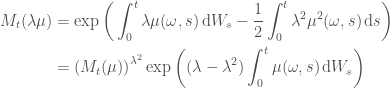
$\displaystyle \begin{aligned} \mathbb{E}((M_t(\lambda\mu))^p) &= \mathbb{E}\bigg[{(M_t(\mu))}^{p\lambda^2}\exp{\bigg(p(\lambda - \lambda^2)\int^t_0 \mu(\omega, s)\,\mathrm{d}W_s\bigg)}\bigg] \\ &\le \bigg|\bigg|{M_t(\mu)}^{p\lambda^2}\bigg|\bigg|_{p\lambda^2} \bigg|\bigg|\exp{\bigg(p(\lambda - \lambda^2)\int^t_0 \mu(\omega, s)\,\mathrm{d}W_s\bigg)}\bigg|\bigg|_{1 - p\lambda^2} \\ &= \mathbb{E}{\bigg[M_t(\mu)}\bigg]^{p\lambda^2} \mathbb{E}\bigg[\exp{\bigg(p\frac{\lambda - \lambda^2}{1 - p\lambda^2}\int^t_0 \mu(\omega, s)\,\mathrm{d}W_s\bigg)}\bigg]^{1 - p\lambda^2} \end{aligned}$

Now let us choose

$\displaystyle p\frac{\lambda - \lambda^2}{1 - p\lambda^2} = \frac{1}{2}$

then

$\displaystyle \begin{aligned} 2p(\lambda - \lambda^2) &= 1 - p\lambda^2 \\ p & = \frac{1}{2(\lambda - \lambda^2) + \lambda^2} \\ p &= \frac{1}{(2 - \lambda)\lambda} \end{aligned}$

In order to apply Hölder’s inequality we need to check that $(p\lambda^2)^{-1} > 1$ and that $(1 - p\lambda^2)^{-1} > 1$ but this amounts to checking that $p\lambda^2 > 0$ and that $1 > \lambda$ . We also need to check that $p > 0$ but this amounts to checking that $(2 - \lambda)\lambda < 1$ for $0 < \lambda < 1$ and this is easily checked to be true.

Re-writing the above inequality with this value of $p$ we have

$\displaystyle \begin{aligned} \mathbb{E}((M_t(\lambda\mu))^p) &\le \mathbb{E}{\bigg[M_t(\mu)}\bigg]^{p\lambda^2} \mathbb{E}\bigg[\exp{\bigg(\frac{1}{2}\int^t_0 \mu(\omega, s)\,\mathrm{d}W_s\bigg)}\bigg]^{1 - p\lambda^2} \end{aligned}$

By the first lemma, since $M_t(\mu)$ is a non-negative local martingale, it is also a supermartingale. Furthermore $\mathbb{E}(M_0(\mu)) = 1$ . Thus

$\displaystyle \mathbb{E}{\bigg[M_t(\mu)}\bigg]^{p\lambda^2} \leq 1$

and therefore

$\displaystyle \begin{aligned} \mathbb{E}((M_t(\lambda\mu))^p) &\le \mathbb{E}\bigg[\exp{\bigg(\frac{1}{2}\int^t_0 \mu(\omega, s)\,\mathrm{d}W_s\bigg)}\bigg]^{1 - p\lambda^2} \end{aligned}$

Step 2

Recall we have

$\displaystyle {M_t} = \exp\bigg( \int_0^t \mu(\omega ,s)\,\mathrm{d}W_s - \frac{1}{2}\int_0^t \mu(\omega ,s)\,\mathrm{d}s \bigg)$

Taking logs gives

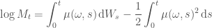
$\displaystyle \log{M_t} = \int_0^t \mu(\omega ,s)\,\mathrm{d}W_s - \frac{1}{2}\int_0^t \mu(\omega ,s)^2\,\mathrm{d}s$

or in diferential form

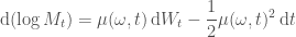
$\displaystyle \mathrm{d}(\log{M_t}) = \mu(\omega ,t)\,\mathrm{d}W_t - \frac{1}{2}\mu(\omega ,t)^2\,\mathrm{d}t$

We can also apply Itô’s rule to $\log{M_t}$

$\displaystyle \begin{aligned} \mathrm{d}(\log{M_t}) &= \frac{1}{M_t}\,\mathrm{d}M_t - \frac{1}{2}\frac{1}{M_t^2}\,\mathrm{d}[M]_t \\ \end{aligned}$

where $[\ldots]$ denotes the quadratic variation of a stochastic process.

Comparing terms gives the stochastic differential equation

$\displaystyle \mathrm{d}M_t = M_t\mu(\omega,t)\,\mathrm{d}W_t$

In integral form this can also be written as

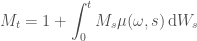
$\displaystyle M_t = 1 + \int_0^t M_s\mu(\omega, s)\,\mathrm{d}W_s$

Thus $M_t$ is a local martingale (it is defined by a stochastic differential equation) and by the first lemma it is a supermaringale. Hence $\mathbb{E}M_t \leq 1$ .

Next we note that

$\displaystyle \exp{\bigg(\frac{1}{2}\int_0^t \mu(\omega, t)\bigg)} = \exp{\bigg(\frac{1}{2}\int_0^t \mu(\omega, t) - \frac{1}{4}\int_0^t \mu^2(\omega, t) \,\mathrm{d}s\bigg)} \exp{\bigg(\frac{1}{4}\int_0^t \mu^2(\omega, t) \,\mathrm{d}s\bigg)}$

to which we can apply Hölder’s inequality with conjugates $p = q = 2$ to obtain

$\displaystyle \begin{aligned} \mathbb{E}\bigg[\exp{\bigg(\frac{1}{2}\int_0^t \mu(\omega, t)\bigg)}\bigg] &= \mathbb{E}\bigg[\exp{\bigg(\frac{1}{2}\int_0^t \mu(\omega, t) - \frac{1}{4}\int_0^t \mu^2(\omega, t) \,\mathrm{d}s \bigg)} \exp{\bigg(\frac{1}{4}\int_0^t \mu^2(\omega, t) \,\mathrm{d}s \bigg)}\bigg] \\ & \leq \sqrt{\mathbb{E}\bigg[\exp{\bigg(\int_0^t \mu(\omega, t) - \frac{1}{2}\int_0^t \mu^2(\omega, t) \,\mathrm{d}s \bigg)}\bigg]} \sqrt{\mathbb{E}\exp{\bigg(\frac{1}{2}\int_0^t \mu^2(\omega, t) \,\mathrm{d}s \bigg)}\bigg]} \end{aligned}$

Applying the supermartingale inequality then gives

$\displaystyle \begin{aligned} \mathbb{E}\bigg[\exp{\bigg(\frac{1}{2}\int_0^t \mu(\omega, t)\bigg)}\bigg] & \leq \sqrt{\mathbb{E}\exp{\bigg(\frac{1}{2}\int_0^t \mu^2(\omega, t) \,\mathrm{d}s \bigg)}\bigg]} \end{aligned}$

Step 3

Now we can apply the result in Step 2 to the result in Step 1.

$\displaystyle \begin{aligned} \mathbb{E}((M_t(\lambda\mu))^p) &\le \mathbb{E}\bigg[\exp{\bigg(\frac{1}{2}\int^t_0 \mu(\omega, s)\,\mathrm{d}W_s\bigg)}\bigg]^{1 - p\lambda^2} \\ &\le {\mathbb{E}\bigg[\exp{\bigg(\frac{1}{2}\int_0^t \mu^2(\omega, t) \,\mathrm{d}s \bigg)}\bigg]}^{(1 - p\lambda^2)/2} \\ &\le K^{(1 - p\lambda^2)/2} \end{aligned}$

We can replace $M_t$ by $M_t {\mathcal{I}}_{t < \tau}$ for any stopping time $\tau$ . Thus for a localizing sequence we have

$\displaystyle \begin{aligned} \mathbb{E}((M_{t \land \tau_n}(\lambda\mu))^p) &\le K^{(1 - p\lambda^2)/2} \end{aligned}$

From which we can conclude

$\displaystyle \sup_n \|M_{T \land \tau_n}(\lambda\mu)\|_p < \infty$

Now we can apply the second lemma to conclude that $M_{T \land \tau_n}(\lambda\mu)$ is a strict martingale.

Final Step

We have already calculated that

Now apply Hölder’s inequality with conjugates $p = \lambda^{-2}$ and $q = (1 - \lambda^2)^{-1}$ .

$\displaystyle 1 = \mathbb{E}(M_t(\lambda\mu) \le \mathbb{E}(M_t(\mu))^{\lambda^2}\mathbb{E}{\bigg(}\exp{\bigg(\frac{\lambda}{1 + \lambda}\int^t_0 \mu(\omega, s)\,\mathrm{d}W_s\bigg)}\bigg)^{1 - \lambda^2}$

And then we can apply Jensen’s inequality to the last term on the right hand side with the convex function $x^{(1 + \lambda)/2\lambda}$ .

$\displaystyle 1 \le \mathbb{E}(M_t(\mu))^{\lambda^2} \mathbb{E}{\bigg(}\exp{\bigg(\frac{1}{2}\int^t_0 \mu(\omega, s)\,\mathrm{d}W_s\bigg)}\bigg)^{2\lambda(1- \lambda)}$

Using the inequality we established in Step 2 and the Novikov condition then gives

$\displaystyle 1 \le \mathbb{E}(M_t(\mu))^{\lambda^2} K^{\lambda(1 - \lambda)}$

If we now let $\lambda \nearrow 1$ we see that we must have $1 \le \mathbb{E}(M_t(\mu))$ . We already now that $1 \ge \mathbb{E}(M_t(\mu))$ by the first lemma and so we have finally proved that $M_t(\mu)$ is a martingale.

Notes

We have already used importance sampling and also touched on changes of measure.
Chebyshev’s inequality is usually stated for the second moment but the proof is easily adapted:

$\displaystyle \mathbb P( |X| > u ) = \int 1_{|X| > u} ~d\mathbb P = \frac 1 {u^p} \int u^p 1_{|X| > u} ~d\mathbb P < \frac 1 {u^p} \int |X|^p 1_{|X| > u} ~ d\mathbb P \le \frac 1 {u^p} \mathbb E|X|^p.$

We follow Handel (2007); a similar approach is given in Steele (2001).

Bibliography

Handel, Ramon von. 2007. “Stochastic Calculus, Filtering, and Stochastic Control (Lecture Notes).”

Steele, J.M. 2001. Stochastic Calculus and Financial Applications. Applications of Mathematics. Springer New York. https://books.google.co.uk/books?id=fsgkBAAAQBAJ.

Maths, Stats & Functional Programming

Formerly known as Idontgetoutmuch's Weblog

Girsanov’s Theorem

Introduction

Random Paths

In General

Girsanov’s Theorem

Proof

The Novikov Sufficiency Condition

The Novikov Sufficiency Condition Statement

Lemma 1

Lemma 2

The Novikov Sufficiency Condition Proof

Step 1

Step 2

Step 3

Final Step

Notes

Bibliography

Leave a comment Cancel reply

Introduction

Random Paths

In General

Girsanov’s Theorem

Proof

The Novikov Sufficiency Condition

The Novikov Sufficiency Condition Statement

Lemma 1

Lemma 2

The Novikov Sufficiency Condition Proof

Step 1

Step 2

Step 3

Final Step

Notes

Bibliography

Related

Leave a comment Cancel reply