Summary
An extended Kalman filter in Haskell using type level literals and automatic differentiation to provide some guarantees of correctness.
Population Growth
Suppose we wish to model population growth of bees via the logistic equation
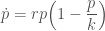
We assume the growth rate 


Haskell Preamble
> {-# OPTIONS_GHC -Wall                     #-}
> {-# OPTIONS_GHC -fno-warn-name-shadowing  #-}
> {-# OPTIONS_GHC -fno-warn-type-defaults   #-}
> {-# OPTIONS_GHC -fno-warn-unused-do-bind  #-}
> {-# OPTIONS_GHC -fno-warn-missing-methods #-}
> {-# OPTIONS_GHC -fno-warn-orphans         #-}
> {-# LANGUAGE DataKinds                    #-}
> {-# LANGUAGE ScopedTypeVariables          #-}
> {-# LANGUAGE RankNTypes                   #-}
> {-# LANGUAGE BangPatterns                 #-}
> {-# LANGUAGE TypeOperators                #-}
> {-# LANGUAGE TypeFamilies                 #-}
> module FunWithKalman3 where
> import GHC.TypeLits
> import Numeric.LinearAlgebra.Static
> import Data.Maybe ( fromJust )
> import Numeric.AD
> import Data.Random.Source.PureMT
> import Data.Random
> import Control.Monad.State
> import qualified Control.Monad.Writer as W
> import Control.Monad.Loops
Logistic Equation
The logistic equation is a well known example of a dynamical system which has an analytic solution
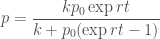
Here it is in Haskell
> logit :: Floating a => a -> a -> a -> a
> logit p0 k x = k * p0 * (exp x) / (k + p0 * (exp x - 1))
We observe a noisy value of population at regular time intervals (where 

Using the semi-group property of our dynamical system, we can re-write this as
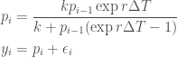
To convince yourself that this re-formulation is correct, think of the population as starting at 


> oneStepFrom0, twoStepsFrom0, oneStepFrom1 :: Double
> oneStepFrom0  = logit 0.1 1.0 (1 * 0.1)
> twoStepsFrom0 = logit 0.1 1.0 (1 * 0.2)
> oneStepFrom1  = logit oneStepFrom0 1.0 (1 * 0.1)
ghci> twoStepsFrom0
  0.11949463171139338

ghci> oneStepFrom1
  0.1194946317113934
We would like to infer the growth rate not just be able to predict the population so we need to add another variable to our model.

Extended Kalman
This is almost in the form suitable for estimation using a Kalman filter but the dependency of the state on the previous state is non-linear. We can modify the Kalman filter to create the extended Kalman filter (EKF) by making a linear approximation.
Since the measurement update is trivially linear (even in this more general form), the measurement update step remains unchanged.

By Taylor we have

where 


Applying this at 

Using the same reasoning as we did as for Kalman filters and writing 

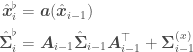
Haskell Implementation
Note that we pass in the Jacobian of the update function as a function itself in the case of the extended Kalman filter rather than the matrix representing the linear function as we do in the case of the classical Kalman filter.
> k, p0 :: Floating a => a
> k = 1.0
> p0 = 0.1 * k
> r, deltaT :: Floating a => a
> r = 10.0
> deltaT = 0.0005
Relating ad and hmatrix is somewhat unpleasant but this can probably be ameliorated by defining a suitable datatype.
> a :: R 2 -> R 2
> a rpPrev = rNew # pNew
>   where
>     (r, pPrev) = headTail rpPrev
>     rNew :: R 1
>     rNew = konst r
>
>     (p,  _) = headTail pPrev
>     pNew :: R 1
>     pNew = fromList $ [logit p k (r * deltaT)]
> bigA :: R 2 -> Sq 2
> bigA rp = fromList $ concat $ j [r, p]
>   where
>     (r, ps) = headTail rp
>     (p,  _) = headTail ps
>     j = jacobian (\[r, p] -> [r, logit p k (r * deltaT)])
For some reason, hmatrix with static guarantees does not yet provide an inverse function for matrices.
> inv :: (KnownNat n, (1 <=? n) ~ 'True) => Sq n -> Sq n
> inv m = fromJust $ linSolve m eye
Here is the extended Kalman filter itself. The type signatures on the expressions inside the function are not necessary but did help the implementor discover a bug in the mathematical derivation and will hopefully help the reader.
> outer ::  forall m n . (KnownNat m, KnownNat n,
>                         (1 <=? n) ~ 'True, (1 <=? m) ~ 'True) =>
>           R n -> Sq n ->
>           L m n -> Sq m ->
>           (R n -> R n) -> (R n -> Sq n) -> Sq n ->
>           [R m] ->
>           [(R n, Sq n)]
> outer muPrior sigmaPrior bigH bigSigmaY
>       littleA bigABuilder bigSigmaX ys = result
>   where
>     result = scanl update (muPrior, sigmaPrior) ys
>
>     update :: (R n, Sq n) -> R m -> (R n, Sq n)
>     update (xHatFlat, bigSigmaHatFlat) y =
>       (xHatFlatNew, bigSigmaHatFlatNew)
>       where
>
>         v :: R m
>         v = y - (bigH #> xHatFlat)
>
>         bigS :: Sq m
>         bigS = bigH <> bigSigmaHatFlat <> (tr bigH) + bigSigmaY
>
>         bigK :: L n m
>         bigK = bigSigmaHatFlat <> (tr bigH) <> (inv bigS)
>
>         xHat :: R n
>         xHat = xHatFlat + bigK #> v
>
>         bigSigmaHat :: Sq n
>         bigSigmaHat = bigSigmaHatFlat - bigK <> bigS <> (tr bigK)
>
>         bigA :: Sq n
>         bigA = bigABuilder xHat
>
>         xHatFlatNew :: R n
>         xHatFlatNew = littleA xHat
>
>         bigSigmaHatFlatNew :: Sq n
>         bigSigmaHatFlatNew = bigA <> bigSigmaHat <> (tr bigA) + bigSigmaX
Now let us create some sample data.
> obsVariance :: Double
> obsVariance = 1e-2
> bigSigmaY :: Sq 1
> bigSigmaY = fromList [obsVariance]
> nObs :: Int
> nObs = 300
> singleSample :: Double -> RVarT (W.Writer [Double]) Double
> singleSample p0 = do
>   epsilon <- rvarT (Normal 0.0 obsVariance)
>   let p1 = logit p0 k (r * deltaT)
>   lift $ W.tell [p1 + epsilon]
>   return p1
> streamSample :: RVarT (W.Writer [Double]) Double
> streamSample = iterateM_ singleSample p0
> samples :: [Double]
> samples = take nObs $ snd $
>           W.runWriter (evalStateT (sample streamSample) (pureMT 3))

We created our data with a growth rate of
ghci> r
  10.0
but let us pretend that we have read the literature on growth rates of bee colonies and we have some big doubts about growth rates but we are almost certain about the size of the colony at 
> muPrior :: R 2
> muPrior = fromList [5.0, 0.1]
>
> sigmaPrior :: Sq 2
> sigmaPrior = fromList [ 1e2, 0.0
>                       , 0.0, 1e-10
>                       ]
We only observe the population and not the rate itself.
> bigH :: L 1 2
> bigH = fromList [0.0, 1.0]
Strictly speaking this should be 0 but this is close enough.
> bigSigmaX :: Sq 2
> bigSigmaX = fromList [ 1e-10, 0.0
>                      , 0.0, 1e-10
>                      ]
Now we can run our filter and watch it switch away from our prior belief as it accumulates more and more evidence.
> test :: [(R 2, Sq 2)]
> test = outer muPrior sigmaPrior bigH bigSigmaY
>        a bigA bigSigmaX (map (fromList . return) samples)


Pingback: Population Growth Estimation via Markov Chain Monte Carlo | Idontgetoutmuch's Weblog