Parallelising Path Dependent Options in Haskell

Path Dependency

Now we are able to price options using parallelism, let us consider a more exotic financial option.

Let us suppose that we wish to price an Asian call option. The payoff at time $T$ is

$\displaystyle {\Bigg(\frac{\Sigma_{i=1}^n x_{t_i}}{n} -k\Bigg)}^+$

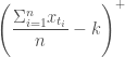
Thus the payoff depends not just on the value of the underlying $x$ at time $T$ but also on the path taken. We do not need to know the entire path, just the average at discrete points in time. Thus the payoff is a function of time, the value of the underlying and the average of the underlying sampled at discrete points in time $z(x,a,t)$ .

We can rewrite this equation as a recursive relation:

$\displaystyle a_n = a_{n-1} + \frac{x_n -a_{n-1}}{n}$

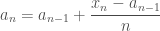
If $t_n$ is the $n$ -th sampling time then for small $\epsilon$ let:

$\begin{aligned}t^+ &= t_n + \epsilon \\t^- &= t_n - \epsilon\end{aligned}$

Now we can write the equation for the value of the average just before and after the sampling time as:

$\displaystyle a(x, t^+) = a(x, t^-) + \frac{x - a(x, t^-)}{n}$

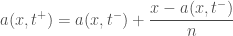
Since there is no arbitrage, the value of the option cannot change as it crosses the sampling date:

$\displaystyle z(x, a^+, t^+) = z(x, a^-, t^-)$

Substituting in:

$\displaystyle z(x, a + (x - a)/n, t^+) = z(x, a, t^-)$

But we have a problem, we do not know the value of $a$ . Away from the sampling times there is no dependence on $a$ as its value cannot change. We already know how to step back in time in this case: we use the pricer we have already developed.

So let us assume a value for $a$ . Then we can diffuse backwards from the final payoff but when we reach a sampling date, we reset the values on the grid using the interfacing formula above.

In summary, we assume a set of values for $a$ and then diffuse backwards for each pricer with that $a$ ; at each sampling time, we reset the values of the pricers and continue until we reach the last sampling time. At this point, $x = a$ so we diffuse one pricer back to the start time which gives us the price of the option for any given $x$ on our grid.

Our usual imports and options.

> {-# LANGUAGE FlexibleContexts          #-}
> {-# LANGUAGE TypeOperators             #-}
> {-# LANGUAGE NoMonomorphismRestriction #-}
> 
> {-# OPTIONS_GHC -Wall                    #-}
> {-# OPTIONS_GHC -fno-warn-name-shadowing #-}
> {-# OPTIONS_GHC -fno-warn-type-defaults  #-}
> 
> import Data.Array.Repa as Repa hiding ((++), map)
> import Control.Monad
> import AsianDiagram
> import Diagrams.Prelude((===))
> import Diagrams.Backend.Cairo.CmdLine
> import Text.Printf
> import Data.List

First some constants for the payoff and the pricer. We make the space grid deliberately coarse so we can draw diagrams showing the grid before and after interfacing.

> r, sigma, k, t, xMax, aMax, deltaX, deltaT, deltaA:: Double
> m, n, p :: Int
> r = 0.05
> sigma = 0.2
> k = 50.0
> t = 3.0
> m = 10
> p = 10
> xMax = 150
> deltaX = xMax / (fromIntegral m)
> aMax = 150
> deltaA = aMax / (fromIntegral p)
> n = 100
> deltaT = t / (fromIntegral n)

We take the times at which do our Asian observations and calculate the number of steps between each observation including the initial and terminal times.

> asianTimes :: [Int]
> asianTimes = map (\x -> floor $ x*(fromIntegral n)/t) [1.5,2.0,2.5]
> 
> numSteps :: [Int]
> numSteps = snd $ mapAccumL (\s x -> (x, x - s)) 0 times
>              where times = asianTimes ++ [n]

As before we can define a single pricer that updates the grid over one time step and at multiple points in space using the Explicit Euler method. We parameterize the upper and lower boundaries $z(0,t)$ and $\lim_{x \to \infty}z(x,t)$ as we will want to use our pricer not just for a vanilla call option.

> type BoundaryCondition = Array D DIM1 Double -> Double
> 
> singleUpdater :: BoundaryCondition ->
>                   BoundaryCondition ->
>                   Array D DIM1 Double ->
>                   Array D DIM1 Double
> singleUpdater lb ub arr = traverse arr id f
>   where
>     Z :. m = extent arr
>     f _get (Z :. ix) | ix == 0   = lb arr
>     f _get (Z :. ix) | ix == m-1 = ub arr
>     f  get (Z :. ix)             = a * get (Z :. ix-1) +
>                                    b * get (Z :. ix) +
>                                    c * get (Z :. ix+1)
>       where
>         a = deltaT * (sigma^2 * x^2 - r * x) / 2
>         b = 1 - deltaT * (r  + sigma^2 * x^2)
>         c = deltaT * (sigma^2 * x^2 + r * x) / 2
>         x = fromIntegral ix

Again we can extend this to update many pricers on one time step and multiple points in space.

> multiUpdater :: Source r Double =>
>                 BoundaryCondition ->
>                 BoundaryCondition ->
>                 Array r DIM2 Double ->
>                 Array D DIM2 Double
> multiUpdater lb ub arr = fromFunction (extent arr) f
>      where
>        f :: DIM2 -> Double
>        f (Z :. ix :. jx) = (singleUpdater lb ub x)!(Z :. ix)
>          where
>            x :: Array D DIM1 Double
>            x = slice arr (Any :. jx)

We define the boundary condition at the maturity date of our Asian option. Notice for each pricer the boundary condition is constant, this being determined by the value of the Asian payoff.

> priceAtTAsian :: Array U DIM2 Double
> priceAtTAsian = fromListUnboxed (Z :. m+1 :. p+1)
>                 [ max 0 (deltaA * (fromIntegral l) - k)
>                 | _j <- [0..m],
>                    l <- [0..p]
>                 ]

With this we can step backwards in time for any number of timesteps.

> stepMulti :: Monad m =>
>              Int ->
>              BoundaryCondition ->
>              BoundaryCondition ->
>              Array U DIM2 Double ->
>              m (Array U DIM2 Double)
> stepMulti n lb ub = updaterM
>   where
>     updaterM :: Monad m => Array U DIM2 Double ->
>                            m (Array U DIM2 Double)
>     updaterM = foldr (>=>) return updaters
>       where
>         updaters = replicate n (computeP . multiUpdater lb ub)

Boundary Conditions

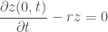
But now we are stuck. What are the boundary conditions for each of the pricers after we have done our interfacing? We follow many practioners and assume that the underlying is linear in this area. Thus in the Black-Scholes equation

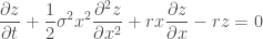
$\displaystyle \frac{\partial z}{\partial t} + \frac{1}{2}\sigma^2 x^2 \frac{\partial^2 z}{\partial x^2} + r x\frac{\partial z}{\partial x} - rz = 0$

we set the second derivative to $0$ . Thus we can use a forward method at the boundary to solve the equation below.

$\displaystyle \frac{\partial z}{\partial t} + r x\frac{\partial z}{\partial x} - rz = 0$

When $x=0$ , we have a simpler situation.

$\displaystyle \frac{\partial z(0,t)}{\partial t} - rz = 0$

The corresponding difference equation for the lower boundary is:

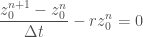
$\displaystyle \frac{z_0^{n+1} - z_0^n}{\Delta t} -rz_0^n = 0$

Which is easily represented in Haskell (rembering we are stepping backwards in time).

> lBoundaryUpdater :: BoundaryCondition
> lBoundaryUpdater arr = x - deltaT * r * x
>   where
>     x = arr!(Z :. (0 :: Int))

The corresponding difference equation for the upper boundary is:

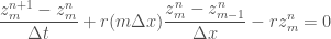
$\displaystyle \frac{z^{n+1}_m - z^n_m}{\Delta t} + r(m\Delta x)\frac{z^n_m - z^n_{m-1}}{\Delta x} - rz^n_m = 0$

Re-arranging

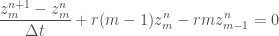
$\displaystyle \frac{z^{n+1}_m - z^n_m}{\Delta t} + r (m-1) z^n_m - r m z^n_{m-1} = 0$

We can write this in Haskell as follows (again remembering we are stepping backwards in time).

> uBoundaryUpdater :: BoundaryCondition
> uBoundaryUpdater arr = x - deltaT * r * (a - b)
>   where
>     Z :. m = extent arr
>     x = arr!(Z :. m - 1)
>     y = arr!(Z :. m - 2)
>     a = x * fromIntegral (m - 1)
>     b = y * fromIntegral m

Interfacing

We interface by linear interpolation if value we require lies between 2 points on our grid otherwise we use linear extrapolation.

> interface :: Int -> Array U DIM2 Double ->
>              Array D DIM2 Double
> interface n grid = traverse grid id (\_ sh -> f sh)
>   where
>     (Z :. _iMax :. jMax) = extent grid
>     f (Z :. i :. j) = inter
>       where
>         x       = deltaX * (fromIntegral i)
>         aPlus   = deltaA * (fromIntegral j)
>         aMinus  = aPlus + (x - aPlus) / (fromIntegral n)
>         jLower  = if k > jMax - 1 then jMax - 1 else k
>                     where k = floor $ aMinus / deltaA
>         jUpper  = if (jLower == jMax - 1)
>                     then jMax - 1
>                     else jLower + 1
>         aLower  = deltaA * (fromIntegral jLower)
>         prptn   = (aMinus - aLower) / deltaA
>         vLower  = grid!(Z :. i :. jLower)
>         vUpper  = grid!(Z :. i :. jUpper)
>         inter   = vLower + prptn * (vUpper - vLower)

Example

Now we are in a position to give an example of pricing our option with a few helper functions

> showD :: Double -> String
> showD = printf "%.2f"
> 
> showArrD1 :: Array U DIM1 Double -> String
> showArrD1 = intercalate ", " . map showD . toList
> 
> showSlices :: String -> Array U DIM2 Double -> IO ()
> showSlices message prices = do
>   putStrLn ('\n' : message)
> 
>   let (Z :. _i :. j) = extent prices
>       slicesD = map (\m -> slice prices (Any :. m)) [0..j-1]
> 
>   slices <- mapM computeP slicesD
>   mapM_ (putStrLn . showArrD1) slices
> 
> diagonal :: Source a Double =>
>             Array a DIM2 Double ->
>             Array D DIM2 Double
> diagonal arr = traverse arr g f
>   where
>     f :: (DIM2 -> Double) -> DIM2 -> Double
>     f get (Z :. ix :. _) = get (Z :. ix :. ix)
> 
>     g :: DIM2 -> DIM2
>     g (Z :. ix :. iy) = Z :. (min ix iy) :. (1 :: Int)
> 
> main :: IO ()
> main = do putStrLn "\nAsianing times"
>           putStrLn $ show asianTimes
> 
>           let lb = lBoundaryUpdater
>               ub = uBoundaryUpdater
> 
>           showSlices "Initial pricers" priceAtTAsian

Now instead of stepping all the way back to the initial time of the option, we only step back to just before the last observation.

>           grid3b <- stepMulti (numSteps!!3) lb ub priceAtTAsian
>           showSlices ("Just before 3") grid3b

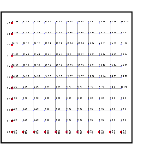
The diagram below shows our grid just before we make the last observation. The $x$ -axis is the value of the underlying and the $y$ -axis is the value of the Asian value. Both have been normalised to 1.0. That is the value 1.0 represents 150.0 (our maximum value on the grid for both the underlying and the Asian / auxiliary variable).

>           grid3a <- computeP $ interface 3 grid3b
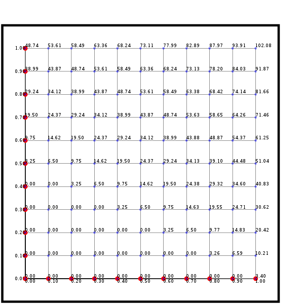
>           showSlices ("Just after 3") grid3a

The diagram below shows our grid after before we make the last observation i.e., after interfacing. Again, the $x$ -axis is the value of the underlying and the $y$ -axis is the value of the Asian value. Both have been normalised to 1.0. That is the value 1.0 represents 150.0 (our maximum value on the grid for both the underlying and the Asian / auxiliary variable).

And then step backwards with the new final boundary condition.

>           grid2b <- stepMulti (numSteps!!2) lb ub grid3a
>           showSlices ("Just before 2") grid2b
> 
>           grid2a <- computeP $ interface 2 grid2b
>           showSlices ("Just after 2") grid2a

Again we step backwards in time with a new final boundary condition.

>           grid1b <- stepMulti (numSteps!!1) lb ub grid2a
>           showSlices ("Just before 1") grid1b

Finally we step all the way back to the time at which we wish to know the price. Here the interface condition is just $x=a$ so we can take the diagonal of our grid and diffuse backwards using a single pricer.

>           grid1a <- computeP $ diagonal grid1b
>           showSlices ("Just after 1") grid1a
>           grid1b <- stepMulti (numSteps!!0) lb ub grid1a
>           showSlices "Final pricer" grid1b

Maths, Stats & Functional Programming

Formerly known as Idontgetoutmuch's Weblog

Parallelising Path Dependent Options in Haskell

Path Dependency

Boundary Conditions

Interfacing

Example

One thought on “Parallelising Path Dependent Options in Haskell”

Leave a comment Cancel reply

Path Dependency

Boundary Conditions

Interfacing

Example

Share this:

Related

One thought on “Parallelising Path Dependent Options in Haskell”

Leave a comment Cancel reply