This is a short example of taking a stochastic system, using Fokker-Planck to convert it to a PDES and using SUNDIALS to solve a 2D partial differential equation in Haskell via the hmatrix-sundials library. The example is taken from the C examples that come with the SUNDIALS source. Here’s the full blog.
One Dimensional Heat Equation via SUNDIALS and Haskell
This is a short example of how to use SUNDIALS to solve a simple partial differential equation in Haskell via the hmatrix-sundials library. The example is taken from the C examples that come with the SUNDIALS source. Here’s the full blog. I’ll give a better URL soonish.
Naperian Functors meet surface sea temperatures
Blog post on my new site.
Data Science in Haskell: An example using temperature data from Thailand and Myanmar
Blog post on my new site.
Estimating Parameters in Chaotic Systems
Cartography in Haskell
Introduction
This blog started off life as a blog post on how I use nix but somehow transformed itself into a “how I do data visualisation” blog post. The nix is still here though quietly doing its work in the background.
Suppose you want to analyze your local election results and visualize them using a choropleth but you’d like to use Haskell. You could try using the shapefile package but you will have to do a lot of the heavy lifting yourself (see here for an extended example). But you know folks using R can produce such things in a few lines of code and you also know from experience that unless you are very disciplined large R scripts can quickly become unmaintainable. Can you get the best of both worlds? It seems you can if you use inline-r. But now you have a bit of configuration problem: how do you make sure that all the Haskell packages that you need and all the R packages that you need are available and how can you make sure that your results are reproducible? My answer to use nix.

Acknowledgements
I’d like to thank all my colleagues at Tweag who have had the patience to indulge my questions especially zimbatm and also all folks on the #nixos irc channel.
Downloading and Building
The sources are on github.
You’ll have to build my Include pandoc filter somehow and then
pandoc -s HowIUseNix.lhs --filter=./Include -t markdown+lhs > HowIUseNixExpanded.lhs
BlogLiterately HowIUseNixExpanded.lhs > HowIUseNixExpanded.html
Analysing the Data
Before looking at the .nix file I use, let’s actually analyse the data. First some preamble
> {-# OPTIONS_GHC -Wall                    #-}
> {-# OPTIONS_GHC -fno-warn-unused-do-bind #-}
> {-# LANGUAGE TemplateHaskell   #-}
> {-# LANGUAGE QuasiQuotes       #-}
> {-# LANGUAGE DataKinds         #-}
> {-# LANGUAGE FlexibleContexts  #-}
> {-# LANGUAGE TypeOperators     #-}
> {-# LANGUAGE OverloadedStrings #-}
> import Prelude as P
> import qualified Language.R as R
> import Language.R.QQ
> import System.Directory
> import System.FilePath
> import Control.Monad
> import Data.List (stripPrefix, nub)
> import qualified Data.Foldable as Foldable
> import Frames hiding ( (:&) )
> import Control.Lens
> import qualified Data.FuzzySet as Fuzzy
> import Data.Text (pack, unpack)
> import qualified Control.Foldl as Foldl
> import Pipes.Prelude (fold)
We can scrape the data for the Kington on Thames local elections and put it in a CSV file. Using the Haskell equivalent of data frames / pandas, Frames, we can “read” in the data. I say “read” in quotes because if this were a big data set (it’s not) then it might not fit in memory and we’d have to process it as a stream. I’ve included the sheet in the github repo so you can try reproducing my results.
> tableTypes "ElectionResults" "data/Election Results 2018 v1.csv"
> loadElectionResults :: IO (Frame ElectionResults)
> loadElectionResults = inCoreAoS (readTable "data/Election Results 2018 v1.csv")
We could analyse the data set in order to find the ward (aka electoral district) names but I happen to know them.
> wardNames :: [Text]
> wardNames = [ "Berrylands"
>             , "Norbiton"
>             , "Old Malden"
>             , "Coombe Hill"
>             , "Beverley"
>             , "Chessington North & Hook"
>             , "Tolworth and Hook Rise"
>             , "Coombe Vale"
>             , "St James"
>             , "Tudor"
>             , "Alexandra"
>             , "Canbury"
>             , "Surbiton Hill"
>             , "Chessington South"
>             , "Grove"
>             , "St Marks"
>             ]
We need a query to get both the total number of votes cast in the ward and the number of votes cast for what is now the party which controls the borough. We can create two filters to run in parallel, summing as we go.
> getPartyWard :: Text -> Text -> Foldl.Fold ElectionResults (Int, Int)
> getPartyWard p w =
>   (,) <$> (Foldl.handles (filtered (\x -> x ^. ward == w)) .
>            Foldl.handles votes) Foldl.sum
>       <*> (Foldl.handles (filtered (\x -> x ^. ward == w &&
>                                           x ^. party == p)) .
>            Foldl.handles votes) Foldl.sum
We can combine all the filters and sums into one big query where they all run in parallel.
> getVotes :: Foldl.Fold ElectionResults [(Int, Int)]
> getVotes = sequenceA $ map (getPartyWard "Liberal Democrat") wardNames
I downloaded the geographical data from here but I imagine there are many other sources.
First we read all the shapefiles in the directory we downloaded.
> root :: FilePath
> root = "data/KingstonuponThames"
> main :: IO ()
> main = do
>   ns <- runSafeT $ Foldl.purely fold getVotes (readTable "data/Election Results 2018 v1.csv")
>   let ps :: [Double]
>       ps = map (\(x, y) -> 100.0 * fromIntegral y / fromIntegral x) ns
>   let percentLD = zip (map unpack wardNames) ps
>
>   ds <- getDirectoryContents root
>   let es = filter (\x -> takeExtension x == ".shp") ds
>   let fs = case xs of
>              Nothing -> error "Ward prefix does not match"
>              Just ys -> ys
>            where
>              xs = sequence $
>                   map (fmap dropExtension) $
>                   map (stripPrefix "KingstonuponThames_") es
Sadly, when we get the ward names from the file names they don’t match the ward names in the electoral data sheet. Fortunately, fuzzy matching resolves this problem.
>   rs <- loadElectionResults
>   let wardSet :: Fuzzy.FuzzySet
>       wardSet = Fuzzy.fromList . nub . Foldable.toList . fmap (^. ward) $ rs
>
>   let gs = case sequence $ map (Fuzzy.getOne wardSet) $ map pack fs of
>              Nothing -> error "Ward name and ward filename do not match"
>              Just xs -> xs
Rather than making the colour of each ward vary continuously depending on the percentage share of the vote, let’s create 4 buckets to make it easier to see at a glance how the election results played out.
>   let bucket :: Double -> String
>       bucket x | x < 40    = "whitesmoke"
>                | x < 50    = "yellow1"
>                | x < 60    = "yellow2"
>                | otherwise = "yellow3"
>
>   let cs :: [String]
>       cs = case sequence $ map (\w -> lookup w percentLD) (map unpack gs) of
>              Nothing -> error "Wrong name in table"
>              Just xs -> map bucket xs
Now we move into the world of R, courtesy of inline-r. First we load up the required libraries. Judging by urls like this, it is not always easy to install the R binding to GDAL (Geospatial Data Abstraction Library). But with nix, we don’t even have to use install.packages(...).
>   R.runRegion $ do
>     [r| library(rgdal)   |]
>     [r| library(ggplot2) |]
>     [r| library(dplyr)   |]
Next we create an empty map (I have no idea what this would look like if it were plotted).
> map0 <- [r| ggplot() |]
And now we can fold over the shape data for each ward and its colour to build the basic map we want.
>     mapN <- foldM
>       (\m (f, c) -> do
>           let wward = root </> f
>           shapefileN <- [r| readOGR(wward_hs) |]
>           shapefileN_df <- [r| fortify(shapefileN_hs) |]
>           withColours <- [r| mutate(shapefileN_df_hs, colour=rep(c_hs, nrow(shapefileN_df_hs))) |]
>           [r| m_hs +
>               geom_polygon(data = withColours_hs,
>                            aes(x = long, y = lat, group = group, fill=colour),
>                            color = 'gray', size = .2) |]) map0 (zip es cs)
Now we can annotate the map with all the details needed to make it intelligible.
>     map_projected <- [r| mapN_hs + coord_map() +
>                          ggtitle("Kingston on Thames 2018 Local Election\nLib Dem Percentage Vote by Ward") +
>                          theme(legend.position="bottom", plot.title = element_text(lineheight=.8, face="bold", hjust=0.5)) +
>                          scale_fill_manual(values=c("whitesmoke", "yellow1", "yellow2", "yellow3"),
>                                            name="Vote (%)",
>                                            labels=c("0%-40% Lib Dem", "40%-50% Lib Dem", "50%-60% Lib Dem", "60%-100% Lib Dem")) |]
And finally save it in a file.
>     [r| jpeg(filename="diagrams/kingston.jpg") |]
>     [r| print(map_projected_hs)               |]
>     [r| dev.off()                             |]
>     return ()
How I Really Use nix
I haven’t found a way of interspersing text with nix code so here are some comments.
-
I use neither all the Haskell packages listed nor all the R packages. I tend to put a shell.nix file in the directory where I am working and then
nix-shell shell.nix -I nixpkgs=~/nixpkgsas at the moment I seem to need packages which were recently added to nixpkgs. -
I couldn’t get the tests for
inline-rto run on MACos so I addeddontCheck. -
Some Haskell packages in nixpkgs have their bounds set too strictly so I have used
doJailbreak.
{ pkgs ? import  {}, compiler ? "ghc822", doBenchmark ? false }:

let

f = { mkDerivation, haskell, base, foldl, Frames, fuzzyset
    , inline-r, integration, lens
    , pandoc-types, plots
    , diagrams-rasterific
    , diagrams
    , diagrams-svg
    , diagrams-contrib
    , R, random, stdenv
    , template-haskell, temporary }:
mkDerivation {
  pname = "mrp";
  version = "1.0.0";
  src = ./.;
  isLibrary = false;
  isExecutable = true;
  executableHaskellDepends = [
    base
    diagrams
    diagrams-rasterific
    diagrams-svg
    diagrams-contrib
    (haskell.lib.dontCheck inline-r)
    foldl
    Frames
    fuzzyset
    integration
    lens
    pandoc-types
    plots
    random
    template-haskell
    temporary
  ];
  executableSystemDepends = [
    R
    pkgs.rPackages.dplyr
    pkgs.rPackages.ggmap
    pkgs.rPackages.ggplot2
    pkgs.rPackages.knitr
    pkgs.rPackages.maptools
    pkgs.rPackages.reshape2
    pkgs.rPackages.rgeos
    pkgs.rPackages.rgdal
    pkgs.rPackages.rstan
    pkgs.rPackages.zoo];
  license = stdenv.lib.licenses.bsd3;
};

haskellPackages = if compiler == "default"
  then pkgs.haskellPackages
  else pkgs.haskell.packages.${compiler};

myHaskellPackages = haskellPackages.override {
  overrides = self: super: with pkgs.haskell.lib; {
    diagrams-rasterific = doJailbreak super.diagrams-rasterific;
    diagrams-svg = doJailbreak super.diagrams-svg;
    diagrams-contrib = doJailbreak super.diagrams-contrib;
    diagrams = doJailbreak super.diagrams;
    inline-r = dontCheck super.inline-r;
    pipes-group = doJailbreak super.pipes-group;
  };
};

variant = if doBenchmark then pkgs.haskell.lib.doBenchmark else pkgs.lib.id;

drv = variant (myHaskellPackages.callPackage f {});

in

  if pkgs.lib.inNixShell then drv.env else drv
Workshop on Numerical Programming in Functional Languages (NPFL)
I’m the chair this year for the first(!) ACM SIGPLAN International
Workshop on Numerical Programming in Functional Languages (NPFL),
which will be co-located with ICFP this September in St. Louis,
Missouri, USA.
Please consider submitting something! All you have to do is submit
between half a page and a page describing your talk. There will be no
proceedings so all you need do is prepare your slides or demo. We do
plan to video the talks for the benefit of the wider world.
We have Eva Darulova giving the keynote.
The submission deadline is Friday 13th July but I and the Committee
would love to see your proposals earlier.
See here for more information. Please contact me if you have any
questions!
Implicit Runge Kutta and GNU Scientific Library
Introduction
These are some very hasty notes on Runge-Kutta methods and IRK2 in particular. I make no apologies for missing lots of details. I may try and put these in a more digestible form but not today.
Some Uncomprehensive Theory
In general, an implicit Runge-Kutta method is given by
where

and
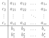
Traditionally this is written as a Butcher tableau:
and even more succintly as

For a Gauß-Legendre method we set the values of the 
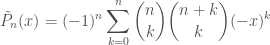
An explicit expression for the shifted Legendre polynomials is given by
The first few shifted Legendre polynomials are:
Setting
then the co-location method gives

For 


that is, the implicit RK2 method aka the mid-point method.
For 


that is, the implicit RK4 method.
Implicit RK2
Explicitly
where

Substituting in the values from the tableau, we have
where
and further inlining and substitution gives
which can be recognised as the mid-point method.
Implementation
A common package for solving ODEs is gsl which Haskell interfaces via the hmatrix-gsl package. Some of gsl is coded with the conditional compilation flag DEBUG e.g. in msbdf.c but sadly not in the simpler methods maybe because they were made part of the package some years earlier. We can add our own of course; here’s a link for reference.
Let’s see how the Implicit Runge-Kutta Order 2 method does on the following system taken from the gsl documenation
which can be re-written as
but replacing gsl_odeiv2_step_rk8pd with gsl_odeiv2_step_rk2imp.
Here’s the first few steps
rk2imp_apply: t=0.00000e+00, h=1.00000e-06, y:1.00000e+00 0.00000e+00
-- evaluate jacobian
(  2,  2)[0,0]:                      0
(  2,  2)[0,1]:                      1
(  2,  2)[1,0]:                     -1
(  2,  2)[1,1]:                     -0
YZ:1.00000e+00 -5.00000e-07
-- error estimates: 0.00000e+00 8.35739e-20
rk2imp_apply: t=1.00000e-06, h=5.00000e-06, y:1.00000e+00 -1.00000e-06
-- evaluate jacobian
(  2,  2)[0,0]:                      0
(  2,  2)[0,1]:                      1
(  2,  2)[1,0]:   -0.99997999999999998
(  2,  2)[1,1]: 1.00008890058234101e-11
YZ:1.00000e+00 -3.50000e-06
-- error estimates: 1.48030e-16 1.04162e-17
rk2imp_apply: t=6.00000e-06, h=2.50000e-05, y:1.00000e+00 -6.00000e-06
-- evaluate jacobian
(  2,  2)[0,0]:                      0
(  2,  2)[0,1]:                      1
(  2,  2)[1,0]:  -0.999880000000002878
(  2,  2)[1,1]: 3.59998697518904009e-10
YZ:1.00000e+00 -1.85000e-05
-- error estimates: 1.48030e-16 1.30208e-15
rk2imp_apply: t=3.10000e-05, h=1.25000e-04, y:1.00000e+00 -3.10000e-05
-- evaluate jacobian
(  2,  2)[0,0]:                      0
(  2,  2)[0,1]:                      1
(  2,  2)[1,0]:  -0.999380000000403723
(  2,  2)[1,1]: 9.6099972424212865e-09
YZ:1.00000e+00 -9.35000e-05
-- error estimates: 0.00000e+00 1.62760e-13
rk2imp_apply: t=1.56000e-04, h=6.25000e-04, y:1.00000e+00 -1.56000e-04
-- evaluate jacobian
(  2,  2)[0,0]:                      0
(  2,  2)[0,1]:                      1
(  2,  2)[1,0]:  -0.996880000051409643
(  2,  2)[1,1]: 2.4335999548874554e-07
YZ:1.00000e+00 -4.68500e-04
-- error estimates: 1.55431e-14 2.03450e-11
Let’s see if we can reproduce this in a fast and loose way in Haskell
To make our code easier to write and read let’s lift some arithmetic operators to act on lists (we should really use the Naperian package).
> module RK2Imp where
> instance Num a => Num [a] where
>   (+) = zipWith (+)
>   (*) = zipWith (*)
The actual algorithm is almost trivial
> rk2Step :: Fractional a => a -> a -> [a] -> [a] -> [a]
> rk2Step h t y_n0 y_n1 = y_n0 + (repeat h) * f (t + 0.5 * h) ((repeat 0.5) * (y_n0 + y_n1))
The example Van der Pol oscillator with the same parameter and initial conditions as in the gsl example.
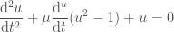
> f :: Fractional b => a -> [b] -> [b]
> f t [y0, y1] = [y1, -y0 - mu * y1 * (y0 * y0 - 1)]
>   where
>     mu = 10.0
> y_init :: [Double]
> y_init = [1.0, 0.0]
We can use co-recursion to find the fixed point of the Runge-Kutta equation arbitrarily choosing the 10th iteration!
> y_1s, y_2s, y_3s :: [[Double]]
> y_1s = y_init : map (rk2Step 1.0e-6 0.0 y_init) y_1s
> nC :: Int
> nC = 10
> y_1, y_2, y_3 :: [Double]
> y_1 = y_1s !! nC
This gives
ghci> y_1
  [0.9999999999995,-9.999999999997499e-7]
which is not too far from the value given by gsl.
y:1.00000e+00 -1.00000e-06 Getting the next time and step size from the gsl DEBUG information we can continue
> y_2s = y_1 : map (rk2Step 5.0e-6 1.0e-6 y_1) y_2s
>
> y_2 = y_2s !! nC
ghci> y_2
  [0.999999999982,-5.999999999953503e-6]
gsl gives
y:1.00000e+00 -6.00000e-06> y_3s = y_2 : map (rk2Step 2.5e-5 6.0e-6 y_2) y_3s
> y_3 = y_3s !! nC
One more time
ghci> y_3
  [0.9999999995194999,-3.099999999372456e-5]
And gsl gives
y:1.00000e+00 -3.10000e-05Nix
The nix-shell which to run this is here and the C code can be built using something like
gcc ode.c -lgsl -lgslcblas -o ode(in the nix shell).
The Haskell code can be used inside a ghci session.
Reproducibility and Old Faithful
Introduction
For the blog post still being written on variatonal methods, I referred to the still excellent Bishop (2006) who uses as his example data, the data available in R for the geyser in Yellowstone National Park called “Old Faithful”.
While explaining this to another statistician, they started to ask about the dataset. Since I couldn’t immediately answer their questions (when was it collected? over how long? how was it collected?), I started to look at the dataset more closely. The more I dug into where the data came from, the less certain I became that the dataset actually reflected how Old Faithful actually behaves.
Here’s what I found. On the way, I use Haskell, R embedded in Haskell, data frames in Haskell and nix.
The Investigation
First some imports and language extensions.
> {-# OPTIONS_GHC -Wall                      #-}
> {-# OPTIONS_GHC -fno-warn-unused-top-binds #-}
>
> {-# LANGUAGE QuasiQuotes          #-}
> {-# LANGUAGE ScopedTypeVariables  #-}
> {-# LANGUAGE DataKinds            #-}
> {-# LANGUAGE FlexibleContexts     #-}
> {-# LANGUAGE TemplateHaskell      #-}
> {-# LANGUAGE TypeOperators        #-}
> {-# LANGUAGE TypeSynonymInstances #-}
> {-# LANGUAGE FlexibleInstances    #-}
> {-# LANGUAGE QuasiQuotes          #-}
> {-# LANGUAGE UndecidableInstances #-}
> {-# LANGUAGE ExplicitForAll       #-}
> {-# LANGUAGE ScopedTypeVariables  #-}
> {-# LANGUAGE OverloadedStrings    #-}
> {-# LANGUAGE GADTs                #-}
> {-# LANGUAGE TypeApplications     #-}
>
>
> module Main (main) where
>
> import Prelude as P
>
> import Control.Lens
>
> import Data.Foldable
> import Frames hiding ( (:&) )
>
> import Data.Vinyl (Rec(..))
>
> import qualified Language.R as R
> import Language.R (R)
> import Language.R.QQ
> import Data.Int
>
> import Plots as P
> import qualified Diagrams.Prelude as D
> import Diagrams.Backend.Rasterific
>
> import Data.Time.Clock(UTCTime, NominalDiffTime, diffUTCTime)
> import Data.Time.Clock.POSIX(posixSecondsToUTCTime)
>
> import Data.Attoparsec.Text
> import Control.Applicative
R provides many datasets presumably for ease of use. We can access the “Old Faithful” data set in Haskell using some very simple inline R.
> eRs :: R s [Double]
> eRs = R.dynSEXP <$> [r| faithful$eruptions |]
>
> wRs :: R s [Int32]
> wRs = R.dynSEXP <$> [r| faithful$waiting |]
And then plot the dataset using
> kSaxis :: [(Double, Double)] -> P.Axis B D.V2 Double
> kSaxis xs = P.r2Axis &~ do
>   P.scatterPlot' xs
>
> plotOF :: IO ()
> plotOF = do
>   es' <- R.runRegion $ do eRs
>   ws' <- R.runRegion $ do wRs
>   renderRasterific "diagrams/Test.png"
>                    (D.dims2D 500.0 500.0)
>                    (renderAxis $ kSaxis $ P.zip es' (P.map fromIntegral ws'))

In the documentation for this dataset, the source is given as Härdle (2012). In here the data are given as a table in Table 3 on page 201. It contains 270 observations not 272 as the R dataset does! Note that there seems to be a correlation between inter-eruption time and duration of eruption and eruptions seem to fall into one of two groups.
The documentation also says “See Also geyser in package MASS for the Azzalini–Bowman version”. So let’s look at this and plot it.
> eAltRs :: R s [Double]
> eAltRs = R.dynSEXP <$> [r| geyser$duration |]
>
> wAltRs :: R s [Int32]
> wAltRs = R.dynSEXP <$> [r| geyser$waiting |]
>
> plotOF' :: IO ()
> plotOF' = do
>   es <- R.runRegion $ do _ <- [r| library(MASS) |]
>                          eAltRs
>   ws <- R.runRegion $ do wAltRs
>   renderRasterific "diagrams/TestR.png"
>                    (D.dims2D 500.0 500.0)
>                    (renderAxis $ kSaxis $ P.zip es (P.map fromIntegral ws))
A quick look at the first few entries suggests this is the data in Table 1 of Azzalini and Bowman (1990) but NB I didn’t check each item.

It looks quite different to the faithful dataset. But to answer my fellow statistician’s questions: “This analysis deals with data which were collected continuously from August 1st until August 15th, 1985”.
It turns out there is a website which collects data for a large number of geysers and has historical datasets for them including old faithful. The data is in a slightly awkward format and it is not clear (to me at any rate) what some of the fields mean.
Let’s examine the first 1000 observations in the data set using the Haskell package Frames.
First we ask Frames to automatically type the data and read it into a frame.
> tableTypes "OldFaithFul" "/Users/dom/Dropbox/Tidy/NumMethHaskell/variational/Old_Faithful_eruptions_1000.csv"
>
> loadOldFaithful :: IO (Frame OldFaithFul)
> loadOldFaithful = inCoreAoS (readTable "/Users/dom/Dropbox/Tidy/NumMethHaskell/variational/Old_Faithful_eruptions_1000.csv")
Declare some columns and helper functions to manipulate the times.
> declareColumn "eruptionTimeNew"  ''UTCTime
> declareColumn "eruptionTimeOld"  ''UTCTime
> declareColumn "eruptionTimeDiff" ''NominalDiffTime
> declareColumn "eruptionTimeRat"  ''Rational
> declareColumn "eruptionTimeDoub" ''Double
> declareColumn "parsedDuration"   ''Double
>
> epochToUTC :: Integral a => a -> UTCTime
> epochToUTC = posixSecondsToUTCTime . fromIntegral
>
> getEruptionTimeNew :: OldFaithFul -> Record '[EruptionTimeNew]
> getEruptionTimeNew x = pure (Col ((epochToUTC (x ^. eruptionTimeEpoch)))) :& Nil
>
> getEruptionTimeOld :: OldFaithFul -> Record '[EruptionTimeOld]
> getEruptionTimeOld x = pure (Col ((epochToUTC (x ^. eruptionTimeEpoch)))) :& Nil
>
> getEruptionTimeDiff :: Record '[EruptionTimeOld, EruptionTimeNew] -> Record '[EruptionTimeDoub]
> getEruptionTimeDiff x = pure (Col ((/60.0) $ fromRational $ toRational $ diffUTCTime (x ^. eruptionTimeNew) (x ^. eruptionTimeOld))) :& Nil
The duration is expressed as a string mainly as e.g. “3.5m” and “3.5min” but occasionally in other formats. Using NaNs to represent data we can’t parse is poor practice but Frames seems to object to types such as Maybe Double.
> getDuration :: OldFaithFul -> Record '["duration" :-> Text]
> getDuration = (rcast @'[Duration])
>
> getParsedDuration :: Record '[Duration, EruptionTimeDoub] -> Record '[ParsedDuration]
> getParsedDuration x = pure (Col ((f $ (parseOnly parseDuration) (x ^. duration)))) :& Nil
>   where
>     f (Left _)  = 0.0 / 0.0
>     f (Right y) = y
>
> parseDuration :: Parser Double
> parseDuration =
>   do d <- double
>      _ <- char 'm'
>      return d
>   <|>
>   do d <- double
>      _ <- string "min"
>      return d
To get the times between eruptions we need to zip the frame with its tail so we define this helper function.
> dropFrame :: Int -> Frame r -> Frame r
> dropFrame n s = Frame ((frameLength s) - 1) (\i -> frameRow s (i + n))
> main :: IO ()
> main = do
>   x <- loadOldFaithful
Get the current eruption times and the previous eruption times and put them in a frame.
>   let tn = dropFrame 1 $ fmap (\b -> (getEruptionTimeNew b)) x
>   let tp = fmap (\b -> (getEruptionTimeOld b)) x
>   let tpns = zipFrames tp tn
Get the durations of the eruptions and exclude any gaps when no observations were taken; arbitrarily if the gap is greate than 1.5 hours.
>   let ds = fmap getDuration x
>   let tds = zipFrames ds (fmap getEruptionTimeDiff tpns)
>   let b = filterFrame (\u -> (u ^. eruptionTimeDoub) <= 150) tds
Parse some of the durations and put the durations and the inter-eruption gap into a single frame.
>   let c = filterFrame (\u -> not $ isNaN $ u ^. parsedDuration) $
>           fmap getParsedDuration b
>   let d = zipFrames b c
>   let g = fmap (\u -> (u ^. parsedDuration, u ^. eruptionTimeDoub)) d
Finally we can yet another data set of observations of old faithful.
>   renderRasterific "diagrams/TestH1000.png"
>                    (D.dims2D 500.0 500.0)
>                    (renderAxis $ kSaxis $ toList g)
>   R.withEmbeddedR R.defaultConfig $ do
>     plotOF
>     plotOF'
>   putStrLn "Finished"

To me this doesn’t look like either of the other two datasets. Perhaps the R faithful data set should be validated, possibly retired and maybe replaced by something with firmer foundations?
Nix
I use nix on MACos for package management both for Haskell and R – no more install.packages problems. Here’s my shell.nix file also available here: here.
{ nixpkgs ? import  {}, compiler ? "ghc822", doBenchmark ? false }:

let

  inherit (nixpkgs) pkgs;

f = { mkDerivation, array, base, bytestring, cassava, containers
    , datasets, diagrams-lib, diagrams-rasterific, foldl, Frames, ghc-prim, hmatrix, hmatrix-gsl
    , inline-r, lens, mtl, pipes, plots, random-fu, R, random-source
    , stdenv, template-haskell, text, typelits-witnesses, vector, vinyl }:
mkDerivation {
  pname = "variational";
  version = "0.1.0.0";
  src = ./.;
  isLibrary = false;
  isExecutable = true;
  executableHaskellDepends = [
    array
    base
    bytestring
    cassava
    containers
    datasets
    diagrams-lib
    diagrams-rasterific
    foldl
    Frames
    ghc-prim
    hmatrix
    inline-r
    lens
    mtl
    pipes
    plots
    random-fu
    random-source
    template-haskell
    text
    typelits-witnesses
    vector
    vinyl
  ];
  executableSystemDepends = [
    R
    pkgs.rPackages.anytime
    pkgs.rPackages.ggplot2
    pkgs.rPackages.maptools
    pkgs.rPackages.reshape2
    pkgs.rPackages.rgeos
    pkgs.rPackages.rgdal
    pkgs.rPackages.rstan ];
  license = stdenv.lib.licenses.bsd3;
};

haskellPackages = if compiler == "default"
  then pkgs.haskellPackages
  else pkgs.haskell.packages.${compiler};

variant = if doBenchmark then pkgs.haskell.lib.doBenchmark else pkgs.lib.id;

drv = variant (haskellPackages.callPackage f {});

in

  if pkgs.lib.inNixShell then drv.env else drv
References
Azzalini, A, and Adrian Bowman. 1990. “Bowman, A.w.: a Look at Some Data on the Old Faithful Geyser. Appl. Stat. 39, 357-365” 39 (January).
Bishop, C.M. 2006. Pattern Recognition and Machine Learning. Information Science and Statistics. Springer. https://books.google.co.uk/books?id=kTNoQgAACAAJ.
Härdle, W. 2012. Smoothing Techniques: With Implementation in S. Springer Series in Statistics. Springer New York. https://books.google.co.uk/books?id=sijUBwAAQBAJ.
Haskell for Numerics?
Introduction
Summary
Back in January, a colleague pointed out to me that GHC did not produce very efficient code for performing floating point abs. I have yet to produce a write-up of my notes about hacking on GHC: in summary it wasn’t as difficult as I had feared and the #ghc folks were extremely helpful.
But maybe getting GHC to produce high performance numerical code is “swimming uphill”. Below is a comparison of a “state of the art” numerical language, Julia, and an alternative Haskell approach, using a Haskell domain-specific embedded language (DSEL), accelerate. The problem is a real one albeit quite simple from a programming point of view and should therefore be taken with some grains of salt.
A bit more background
The reason for improving GHC’s (numerical) performance is that I’d like to have a fast way of performing statistical inference either via Hamiltonian Monte Carlo or Sequential Monte Carlo. Stan is my “go to” tool for offline analysis but its inference engine is fixed and according to Fast Forward Labs: “it’s very awkward to productize”. What one would really like is the ability to choose and compose inference methods like can be done in monad-bayes. Although I haven’t compared monad-bayes and Stan in very much depth, the latter seems faster in my very limited experience.
The view of one of the folks that’s worked hard on making Haskell a great tool for doing numerical applications is that trying to get GHC to produce llvm on which tools like polly can work is “swimming up hill”.
A lot of people who work on numerical problems use matlab but it seems like if you want to put the code into production then you have to re-write it. Julia is an attempt to improve this situation and also provide higher performance.
A sort of manifesto
To summarise: what we’d like is type-safe blazingly fast numerical code. Type-safe can give us e.g. static guarantees that matrix multiplication is between compatible matrices and assurances that the units are correct. Here’s an example of static typing helping ensure the correctness of Kalman filter usage and here’s a package that I have used successfully on a medium-sized project to ensure all units are correct.
Symplectic Integrators
Let’s take a simple solver, encode it in Haskell and Julia and see how well we can do.
> {-# OPTIONS_GHC -Wall                   #-}
> {-# OPTIONS_GHC -fno-warn-type-defaults #-}
>
> {-# LANGUAGE FlexibleContexts #-}
> {-# LANGUAGE TypeOperators    #-}
> module Symplectic (
>     runSteps
>   , runSteps'
>   , reallyRunSteps'
>   , inits
>   , h
>   , bigH1
>   , hs
>   , nabla1
>   , nabla2
>   , runStepsH98
>   , bigH2BodyH98
>   ) where
>
> import Data.Number.Symbolic
> import Numeric.AD
> import Prelude                            as P
> import Data.Array.Accelerate              as A   hiding ((^))
> import Data.Array.Accelerate.LLVM.Native  as CPU
> import Data.Array.Accelerate.Linear              hiding (trace)
> import Data.Array.Accelerate.Control.Lens
> import qualified Linear                   as L
The Störmer-Verlet scheme is an implicit symplectic method of order 2. Being symplectic is important as it preserves the energy of the systems being solved. If, for example, we were to use RK4 to simulate planetary motion then the planets would either crash into the sun or leave the solar system: not a very accurate representation of reality.
Let’s assume that the Hamiltonian is of the form 

Simple Pendulum
Consider the following Hamiltonian for the pendulum:
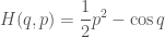
> bigH1 :: P.Floating a => a -> a -> a
> bigH1 q p = p^2 / 2 - cos q
> ham1 :: P.Floating a => [a] -> a
> ham1 [qq1, pp1] = 0.5 * pp1^2 - cos qq1
> ham1 _ = error "Hamiltonian defined for 2 generalized co-ordinates only"
Although it is trivial to find the derivatives in this case, let us check using automatic symbolic differentiation
> q1, q2, p1, p2 :: Sym a
> q1 = var "q1"
> q2 = var "q2"
> p1 = var "p1"
> p2 = var "p2"
> nabla1 :: [[Sym Double]]
> nabla1 = jacobian ((\x -> [x]) . ham1) [q1, p1]
ghci> nabla1
  [[sin q1,0.5*p1+0.5*p1]]
which after a bit of simplification gives us 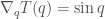

> nablaQ, nablaP :: P.Floating a => a -> a
> nablaQ = sin
> nablaP = id
One step of the Störmer-Verlet
> oneStep :: P.Floating a => (a -> a) ->
>                                  (a -> a) ->
>                                  a ->
>                                  (a, a) ->
>                                  (a, a)
> oneStep nabalQQ nablaPP hh (qPrev, pPrev) = (qNew, pNew)
>   where
>     h2 = hh / 2
>     pp2 = pPrev - h2 * nabalQQ qPrev
>     qNew = qPrev + hh * nablaPP pp2
>     pNew = pp2 - h2 * nabalQQ qNew
> h :: Double
> h = 0.01
> hs :: (Double, Double) -> [(Double, Double)]
> hs = P.iterate (oneStep nablaQ nablaP h)
We can check that the energy is conserved directly
ghci> P.map (P.uncurry bigH1) $ P.take 5 $               hs (pi/4, 0.0)
  [-0.7071067811865476,-0.7071067816284917,-0.7071067829543561,-0.7071067851642338,-0.7071067882582796]

ghci> P.map (P.uncurry bigH1) $ P.take 5 $ P.drop 1000 $ hs (pi/4, 0.0)
  [-0.7071069557227465,-0.7071069737863691,-0.7071069927439544,-0.7071070125961187,-0.7071070333434369]
Two body problem
Newton’s equations of motions for the two body problem are
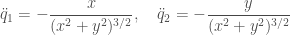
And we can re-write those to use Hamilton’s equations with this Hamiltonian
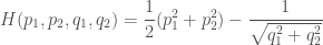
The advantage of using this small example is that we know the exact solution should we need it.
> ham2 :: P.Floating a => [a] -> a
> ham2 [qq1, qq2, pp1, pp2] = 0.5 * (pp1^2 + pp2^2) - recip (sqrt (qq1^2 + qq2^2))
> ham2 _ = error "Hamiltonian defined for 4 generalized co-ordinates only"
Again we can calculate the derivatives
> nabla2 :: [[Sym Double]]
> nabla2 = jacobian ((\x -> [x]) . ham2) [q1, q2, p1, p2]
ghci> (P.mapM_ . P.mapM_) putStrLn . P.map (P.map show) $ nabla2
  q1/(2.0*sqrt (q1*q1+q2*q2))/sqrt (q1*q1+q2*q2)/sqrt (q1*q1+q2*q2)+q1/(2.0*sqrt (q1*q1+q2*q2))/sqrt (q1*q1+q2*q2)/sqrt (q1*q1+q2*q2)
  q2/(2.0*sqrt (q1*q1+q2*q2))/sqrt (q1*q1+q2*q2)/sqrt (q1*q1+q2*q2)+q2/(2.0*sqrt (q1*q1+q2*q2))/sqrt (q1*q1+q2*q2)/sqrt (q1*q1+q2*q2)
  0.5*p1+0.5*p1
  0.5*p2+0.5*p2
which after some simplification becomes

Here’s one step of Störmer-Verlet using Haskell 98.
> oneStepH98 :: Double -> V2 (V2 Double) -> V2 (V2 Double)
> oneStepH98 hh prev = V2 qNew pNew
>   where
>     h2 = hh / 2
>     hhs = V2 hh hh
>     hh2s = V2 h2 h2
>     pp2 = psPrev - hh2s * nablaQ' qsPrev
>     qNew = qsPrev + hhs * nablaP' pp2
>     pNew = pp2 - hh2s * nablaQ' qNew
>     qsPrev = prev ^. L._x
>     psPrev = prev ^. L._y
>     nablaQ' qs = V2 (qq1 / r) (qq2 / r)
>       where
>         qq1 = qs ^. L._x
>         qq2 = qs ^. L._y
>         r   = (qq1 ^ 2 + qq2 ^ 2) ** (3/2)
>     nablaP' ps = ps
And here is the same thing using accelerate.
> oneStep2 :: Double -> Exp (V2 (V2 Double)) -> Exp (V2 (V2 Double))
> oneStep2 hh prev = lift $ V2 qNew pNew
>   where
>     h2 = hh / 2
>     hhs = lift $ V2 hh hh
>     hh2s = lift $ V2 h2 h2
>     pp2 = psPrev - hh2s * nablaQ' qsPrev
>     qNew = qsPrev + hhs * nablaP' pp2
>     pNew = pp2 - hh2s * nablaQ' qNew
>     qsPrev :: Exp (V2 Double)
>     qsPrev = prev ^. _x
>     psPrev = prev ^. _y
>     nablaQ' :: Exp (V2 Double) -> Exp (V2 Double)
>     nablaQ' qs = lift (V2 (qq1 / r) (qq2 / r))
>       where
>         qq1 = qs ^. _x
>         qq2 = qs ^. _y
>         r   = (qq1 ^ 2 + qq2 ^ 2) ** (3/2)
>     nablaP' :: Exp (V2 Double) -> Exp (V2 Double)
>     nablaP' ps = ps
With initial values below the solution is an ellipse with eccentricity 
> e, q10, q20, p10, p20 :: Double
> e = 0.6
> q10 = 1 - e
> q20 = 0.0
> p10 = 0.0
> p20 = sqrt ((1 + e) / (1 - e))
> initsH98 :: V2 (V2 Double)
> initsH98 = V2 (V2 q10 q20) (V2 p10 p20)
>
> inits :: Exp (V2 (V2 Double))
> inits = lift initsH98
We can either keep all the steps of the simulation using accelerate and the CPU
> nSteps :: Int
> nSteps = 10000
>
> dummyInputs :: Acc (Array DIM1 (V2 (V2 Double)))
> dummyInputs = A.use $ A.fromList (Z :. nSteps) $
>                P.replicate nSteps (V2 (V2 0.0 0.0) (V2 0.0 0.0))
> runSteps :: Array DIM1 (V2 (V2 Double))
> runSteps = CPU.run $ A.scanl (\s _x -> (oneStep2 h s)) inits dummyInputs
Or we can do the same in plain Haskell
> dummyInputsH98 :: [V2 (V2 Double)]
> dummyInputsH98 = P.replicate nSteps (V2 (V2 0.0 0.0) (V2 0.0 0.0))
> runStepsH98 :: [V2 (V2 Double)]
> runStepsH98= P.scanl (\s _x -> (oneStepH98 h s)) initsH98 dummyInputsH98
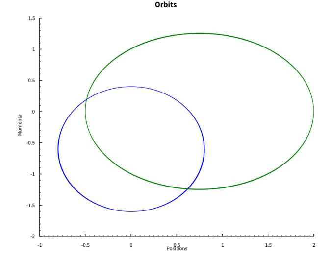
The fact that the phase diagram for the two objects is periodic is encouraging.
And again we can check directly that the energy is conserved.
> bigH2BodyH98 :: V2 (V2 Double) -> Double
> bigH2BodyH98 z = ke + pe
>   where
>     q = z ^. L._x
>     p = z ^. L._y
>     pe = let V2 q1' q2' = q in negate $ recip (sqrt (q1'^2 + q2'^2))
>     ke = let V2 p1' p2' = p in 0.5 * (p1'^2 + p2'^2)
ghci> P.maximum $ P.map bigH2BodyH98 $ P.take 100 $ P.drop 1000 runStepsH98
  -0.49964056333352014

ghci> P.minimum $ P.map bigH2BodyH98 $ P.take 100 $ P.drop 1000 runStepsH98
  -0.49964155784917147
We’d like to measure performance and running the above for many steps might use up all available memory. Let’s confine ourselves to looking at the final result.
> runSteps' :: Int -> Exp (V2 (V2 Double)) -> Exp (V2 (V2 Double))
> runSteps' nSteps = A.iterate (lift nSteps) (oneStep2 h)
> reallyRunSteps' :: Int -> Array DIM1 (V2 (V2 Double))
> reallyRunSteps' nSteps = CPU.run $
>                          A.scanl (\s _x -> runSteps' nSteps s) inits
>                          (A.use $ A.fromList (Z :. 1) [V2 (V2 0.0 0.0) (V2 0.0 0.0)])
Performance
Accelerate’s LLVM
Let’s see what accelerate generates with
{-# OPTIONS_GHC -Wall                      #-}
{-# OPTIONS_GHC -fno-warn-name-shadowing   #-}
{-# OPTIONS_GHC -fno-warn-type-defaults    #-}
{-# OPTIONS_GHC -fno-warn-unused-do-bind   #-}
{-# OPTIONS_GHC -fno-warn-missing-methods  #-}
{-# OPTIONS_GHC -fno-warn-orphans          #-}

import Symplectic

main :: IO ()
main = do
  putStrLn $ show $ reallyRunSteps' 100000000
It’s a bit verbose but we can look at the key “loop”: while5.
[   0.023] llvm: generated 102 instructions in 10 blocks
[   0.023] llvm: generated 127 instructions in 15 blocks
[   0.023] llvm: generated 86 instructions in 7 blocks
[   0.024] llvm: generated 84 instructions in 7 blocks
[   0.024] llvm: generated 18 instructions in 4 blocks
[   0.071] llvm: optimisation did work? True
[   0.072] ; ModuleID = 'scanS'
target datalayout = "e-m:o-i64:64-f80:128-n8:16:32:64-S128"
target triple = "x86_64-apple-darwin15.5.0"

@.memset_pattern = private unnamed_addr constant [2 x double] [double 2.000000e+00, double 2.000000e+00], align 16
@.memset_pattern.1 = private unnamed_addr constant [2 x double] [double 4.000000e-01, double 4.000000e-01], align 16

; Function Attrs: nounwind
define void @scanS(i64 %ix.start, i64 %ix.end, double* noalias nocapture %out.ad3, double* noalias nocapture %out.ad2, double* noalias nocapture %out.ad1, double* noalias nocapture %out.ad0, i64 %out.sh0, double* noalias nocapture readnone %fv0.ad3, double* noalias nocapture readnone %fv0.ad2, double* noalias nocapture readnone %fv0.ad1, double* noalias nocapture readnone %fv0.ad0, i64 %fv0.sh0) local_unnamed_addr #0 {
entry:
  %0 = add i64 %fv0.sh0, 1
  %1 = icmp slt i64 %ix.start, %ix.end
  br i1 %1, label %while1.top.preheader, label %while1.exit

while1.top.preheader:                             ; preds = %entry
  %2 = add i64 %ix.start, 1
  %3 = mul i64 %2, %fv0.sh0
  br label %while1.top

while1.top:                                       ; preds = %while3.exit, %while1.top.preheader
  %indvars.iv = phi i64 [ %3, %while1.top.preheader ], [ %indvars.iv.next, %while3.exit ]
  %4 = phi i64 [ %ix.start, %while1.top.preheader ], [ %52, %while3.exit ]
  %5 = mul i64 %4, %fv0.sh0
  %6 = mul i64 %4, %0
  %7 = getelementptr double, double* %out.ad0, i64 %6
  store double 2.000000e+00, double* %7, align 8
  %8 = getelementptr double, double* %out.ad1, i64 %6
  store double 0.000000e+00, double* %8, align 8
  %9 = getelementptr double, double* %out.ad2, i64 %6
  store double 0.000000e+00, double* %9, align 8
  %10 = getelementptr double, double* %out.ad3, i64 %6
  store double 4.000000e-01, double* %10, align 8
  %11 = add i64 %5, %fv0.sh0
  %12 = icmp slt i64 %5, %11
  br i1 %12, label %while3.top.preheader, label %while3.exit

while3.top.preheader:                             ; preds = %while1.top
  br label %while3.top

while3.top:                                       ; preds = %while3.top.preheader, %while5.exit
  %.in = phi i64 [ %44, %while5.exit ], [ %6, %while3.top.preheader ]
  %13 = phi i64 [ %51, %while5.exit ], [ %5, %while3.top.preheader ]
  %14 = phi <2 x double> [ %43, %while5.exit ], [ <double 2.000000e+00, double 0.000000e+00>, %while3.top.preheader ]
  %15 = phi <2 x double> [ %32, %while5.exit ], [ <double 0.000000e+00, double 4.000000e-01>, %while3.top.preheader ]
  br label %while5.top

while5.top:                                       ; preds = %while5.top, %while3.top
  %16 = phi i64 [ 0, %while3.top ], [ %19, %while5.top ]
  %17 = phi <2 x double> [ %14, %while3.top ], [ %43, %while5.top ]
  %18 = phi <2 x double> [ %15, %while3.top ], [ %32, %while5.top ]
  %19 = add nuw nsw i64 %16, 1
  %20 = extractelement <2 x double> %18, i32 1
  %21 = fmul fast double %20, %20
  %22 = extractelement <2 x double> %18, i32 0
  %23 = fmul fast double %22, %22
  %24 = fadd fast double %21, %23
  %25 = tail call double @llvm.pow.f64(double %24, double 1.500000e+00) #2
  %26 = insertelement <2 x double> undef, double %25, i32 0
  %27 = shufflevector <2 x double> %26, <2 x double> undef, <2 x i32> zeroinitializer
  %28 = fdiv fast <2 x double> %18, %27
  %29 = fmul fast <2 x double> %28, <double 5.000000e-03, double 5.000000e-03>
  %30 = fsub fast <2 x double> %17, %29
  %31 = fmul fast <2 x double> %30, <double 1.000000e-02, double 1.000000e-02>
  %32 = fadd fast <2 x double> %31, %18
  %33 = extractelement <2 x double> %32, i32 1
  %34 = fmul fast double %33, %33
  %35 = extractelement <2 x double> %32, i32 0
  %36 = fmul fast double %35, %35
  %37 = fadd fast double %34, %36
  %38 = tail call double @llvm.pow.f64(double %37, double 1.500000e+00) #2
  %39 = insertelement <2 x double> undef, double %38, i32 0
  %40 = shufflevector <2 x double> %39, <2 x double> undef, <2 x i32> zeroinitializer
  %41 = fdiv fast <2 x double> %32, %40
  %42 = fmul fast <2 x double> %41, <double 5.000000e-03, double 5.000000e-03>
  %43 = fsub fast <2 x double> %30, %42
  %exitcond = icmp eq i64 %19, 100000000
  br i1 %exitcond, label %while5.exit, label %while5.top

while5.exit:                                      ; preds = %while5.top
  %44 = add i64 %.in, 1
  %45 = getelementptr double, double* %out.ad0, i64 %44
  %46 = extractelement <2 x double> %43, i32 0
  store double %46, double* %45, align 8
  %47 = getelementptr double, double* %out.ad1, i64 %44
  %48 = extractelement <2 x double> %43, i32 1
  store double %48, double* %47, align 8
  %49 = getelementptr double, double* %out.ad2, i64 %44
  store double %35, double* %49, align 8
  %50 = getelementptr double, double* %out.ad3, i64 %44
  store double %33, double* %50, align 8
  %51 = add i64 %13, 1
  %exitcond7 = icmp eq i64 %51, %indvars.iv
  br i1 %exitcond7, label %while3.exit.loopexit, label %while3.top

while3.exit.loopexit:                             ; preds = %while5.exit
  br label %while3.exit

while3.exit:                                      ; preds = %while3.exit.loopexit, %while1.top
  %52 = add nsw i64 %4, 1
  %indvars.iv.next = add i64 %indvars.iv, %fv0.sh0
  %exitcond8 = icmp eq i64 %52, %ix.end
  br i1 %exitcond8, label %while1.exit.loopexit, label %while1.top

while1.exit.loopexit:                             ; preds = %while3.exit
  br label %while1.exit

while1.exit:                                      ; preds = %while1.exit.loopexit, %entry
  ret void
}

; Function Attrs: nounwind
define void @scanP1(i64 %ix.start, i64 %ix.end, i64 %ix.stride, i64 %ix.steps, double* noalias nocapture %out.ad3, double* noalias nocapture %out.ad2, double* noalias nocapture %out.ad1, double* noalias nocapture %out.ad0, i64 %out.sh0, double* noalias nocapture %tmp.ad3, double* noalias nocapture %tmp.ad2, double* noalias nocapture %tmp.ad1, double* noalias nocapture %tmp.ad0, i64 %tmp.sh0, double* noalias nocapture readonly %fv0.ad3, double* noalias nocapture readonly %fv0.ad2, double* noalias nocapture readonly %fv0.ad1, double* noalias nocapture readonly %fv0.ad0, i64 %fv0.sh0) local_unnamed_addr #0 {
entry:
  %0 = mul i64 %ix.stride, %ix.start
  %1 = add i64 %0, %ix.stride
  %2 = icmp sle i64 %1, %fv0.sh0
  %3 = select i1 %2, i64 %1, i64 %fv0.sh0
  %4 = icmp eq i64 %ix.start, 0
  %5 = add i64 %0, 1
  %6 = select i1 %4, i64 %0, i64 %5
  br i1 %4, label %if5.exit, label %if5.else

if5.else:                                         ; preds = %entry
  %7 = getelementptr double, double* %fv0.ad3, i64 %0
  %8 = load double, double* %7, align 8
  %9 = getelementptr double, double* %fv0.ad2, i64 %0
  %10 = load double, double* %9, align 8
  %11 = getelementptr double, double* %fv0.ad1, i64 %0
  %12 = load double, double* %11, align 8
  %13 = getelementptr double, double* %fv0.ad0, i64 %0
  %14 = load double, double* %13, align 8
  %15 = insertelement <2 x double> undef, double %14, i32 0
  %16 = insertelement <2 x double> %15, double %12, i32 1
  %17 = insertelement <2 x double> undef, double %10, i32 0
  %18 = insertelement <2 x double> %17, double %8, i32 1
  br label %if5.exit

if5.exit:                                         ; preds = %entry, %if5.else
  %19 = phi i64 [ %5, %if5.else ], [ %0, %entry ]
  %20 = phi <2 x double> [ %16, %if5.else ], [ <double 2.000000e+00, double 0.000000e+00>, %entry ]
  %21 = phi <2 x double> [ %18, %if5.else ], [ <double 0.000000e+00, double 4.000000e-01>, %entry ]
  %22 = getelementptr double, double* %out.ad0, i64 %6
  %23 = extractelement <2 x double> %20, i32 0
  store double %23, double* %22, align 8
  %24 = getelementptr double, double* %out.ad1, i64 %6
  %25 = extractelement <2 x double> %20, i32 1
  store double %25, double* %24, align 8
  %26 = getelementptr double, double* %out.ad2, i64 %6
  %27 = extractelement <2 x double> %21, i32 0
  store double %27, double* %26, align 8
  %28 = getelementptr double, double* %out.ad3, i64 %6
  %29 = extractelement <2 x double> %21, i32 1
  store double %29, double* %28, align 8
  %30 = icmp slt i64 %19, %3
  br i1 %30, label %while9.top.preheader, label %while9.exit

while9.top.preheader:                             ; preds = %if5.exit
  br label %while9.top

while9.top:                                       ; preds = %while9.top.preheader, %while11.exit
  %.in = phi i64 [ %62, %while11.exit ], [ %6, %while9.top.preheader ]
  %31 = phi i64 [ %69, %while11.exit ], [ %19, %while9.top.preheader ]
  %32 = phi <2 x double> [ %61, %while11.exit ], [ %20, %while9.top.preheader ]
  %33 = phi <2 x double> [ %50, %while11.exit ], [ %21, %while9.top.preheader ]
  br label %while11.top

while11.top:                                      ; preds = %while11.top, %while9.top
  %34 = phi i64 [ 0, %while9.top ], [ %37, %while11.top ]
  %35 = phi <2 x double> [ %32, %while9.top ], [ %61, %while11.top ]
  %36 = phi <2 x double> [ %33, %while9.top ], [ %50, %while11.top ]
  %37 = add nuw nsw i64 %34, 1
  %38 = extractelement <2 x double> %36, i32 1
  %39 = fmul fast double %38, %38
  %40 = extractelement <2 x double> %36, i32 0
  %41 = fmul fast double %40, %40
  %42 = fadd fast double %39, %41
  %43 = tail call double @llvm.pow.f64(double %42, double 1.500000e+00) #2
  %44 = insertelement <2 x double> undef, double %43, i32 0
  %45 = shufflevector <2 x double> %44, <2 x double> undef, <2 x i32> zeroinitializer
  %46 = fdiv fast <2 x double> %36, %45
  %47 = fmul fast <2 x double> %46, <double 5.000000e-03, double 5.000000e-03>
  %48 = fsub fast <2 x double> %35, %47
  %49 = fmul fast <2 x double> %48, <double 1.000000e-02, double 1.000000e-02>
  %50 = fadd fast <2 x double> %49, %36
  %51 = extractelement <2 x double> %50, i32 1
  %52 = fmul fast double %51, %51
  %53 = extractelement <2 x double> %50, i32 0
  %54 = fmul fast double %53, %53
  %55 = fadd fast double %52, %54
  %56 = tail call double @llvm.pow.f64(double %55, double 1.500000e+00) #2
  %57 = insertelement <2 x double> undef, double %56, i32 0
  %58 = shufflevector <2 x double> %57, <2 x double> undef, <2 x i32> zeroinitializer
  %59 = fdiv fast <2 x double> %50, %58
  %60 = fmul fast <2 x double> %59, <double 5.000000e-03, double 5.000000e-03>
  %61 = fsub fast <2 x double> %48, %60
  %exitcond = icmp eq i64 %37, 100000000
  br i1 %exitcond, label %while11.exit, label %while11.top

while11.exit:                                     ; preds = %while11.top
  %62 = add i64 %.in, 1
  %63 = getelementptr double, double* %out.ad0, i64 %62
  %64 = extractelement <2 x double> %61, i32 0
  store double %64, double* %63, align 8
  %65 = getelementptr double, double* %out.ad1, i64 %62
  %66 = extractelement <2 x double> %61, i32 1
  store double %66, double* %65, align 8
  %67 = getelementptr double, double* %out.ad2, i64 %62
  store double %53, double* %67, align 8
  %68 = getelementptr double, double* %out.ad3, i64 %62
  store double %51, double* %68, align 8
  %69 = add nsw i64 %31, 1
  %70 = icmp slt i64 %69, %3
  br i1 %70, label %while9.top, label %while9.exit.loopexit

while9.exit.loopexit:                             ; preds = %while11.exit
  br label %while9.exit

while9.exit:                                      ; preds = %while9.exit.loopexit, %if5.exit
  %71 = phi <2 x double> [ %20, %if5.exit ], [ %61, %while9.exit.loopexit ]
  %72 = phi <2 x double> [ %21, %if5.exit ], [ %50, %while9.exit.loopexit ]
  %73 = getelementptr double, double* %tmp.ad0, i64 %ix.start
  %74 = extractelement <2 x double> %71, i32 0
  store double %74, double* %73, align 8
  %75 = getelementptr double, double* %tmp.ad1, i64 %ix.start
  %76 = extractelement <2 x double> %71, i32 1
  store double %76, double* %75, align 8
  %77 = getelementptr double, double* %tmp.ad2, i64 %ix.start
  %78 = extractelement <2 x double> %72, i32 0
  store double %78, double* %77, align 8
  %79 = getelementptr double, double* %tmp.ad3, i64 %ix.start
  %80 = extractelement <2 x double> %72, i32 1
  store double %80, double* %79, align 8
  ret void
}

; Function Attrs: nounwind
define void @scanP2(i64 %ix.start, i64 %ix.end, double* noalias nocapture %tmp.ad3, double* noalias nocapture %tmp.ad2, double* noalias nocapture %tmp.ad1, double* noalias nocapture %tmp.ad0, i64 %tmp.sh0, double* noalias nocapture readnone %fv0.ad3, double* noalias nocapture readnone %fv0.ad2, double* noalias nocapture readnone %fv0.ad1, double* noalias nocapture readnone %fv0.ad0, i64 %fv0.sh0) local_unnamed_addr #0 {
entry:
  %0 = add i64 %ix.start, 1
  %1 = icmp slt i64 %0, %ix.end
  br i1 %1, label %while1.top.preheader, label %while1.exit

while1.top.preheader:                             ; preds = %entry
  %2 = getelementptr double, double* %tmp.ad3, i64 %ix.start
  %3 = load double, double* %2, align 8
  %4 = getelementptr double, double* %tmp.ad2, i64 %ix.start
  %5 = load double, double* %4, align 8
  %6 = getelementptr double, double* %tmp.ad1, i64 %ix.start
  %7 = load double, double* %6, align 8
  %8 = getelementptr double, double* %tmp.ad0, i64 %ix.start
  %9 = load double, double* %8, align 8
  %10 = insertelement <2 x double> undef, double %5, i32 0
  %11 = insertelement <2 x double> %10, double %3, i32 1
  %12 = insertelement <2 x double> undef, double %9, i32 0
  %13 = insertelement <2 x double> %12, double %7, i32 1
  br label %while1.top

while1.top:                                       ; preds = %while3.exit, %while1.top.preheader
  %14 = phi i64 [ %45, %while3.exit ], [ %0, %while1.top.preheader ]
  %15 = phi <2 x double> [ %44, %while3.exit ], [ %13, %while1.top.preheader ]
  %16 = phi <2 x double> [ %33, %while3.exit ], [ %11, %while1.top.preheader ]
  br label %while3.top

while3.top:                                       ; preds = %while3.top, %while1.top
  %17 = phi i64 [ 0, %while1.top ], [ %20, %while3.top ]
  %18 = phi <2 x double> [ %15, %while1.top ], [ %44, %while3.top ]
  %19 = phi <2 x double> [ %16, %while1.top ], [ %33, %while3.top ]
  %20 = add nuw nsw i64 %17, 1
  %21 = extractelement <2 x double> %19, i32 1
  %22 = fmul fast double %21, %21
  %23 = extractelement <2 x double> %19, i32 0
  %24 = fmul fast double %23, %23
  %25 = fadd fast double %22, %24
  %26 = tail call double @llvm.pow.f64(double %25, double 1.500000e+00) #2
  %27 = insertelement <2 x double> undef, double %26, i32 0
  %28 = shufflevector <2 x double> %27, <2 x double> undef, <2 x i32> zeroinitializer
  %29 = fdiv fast <2 x double> %19, %28
  %30 = fmul fast <2 x double> %29, <double 5.000000e-03, double 5.000000e-03>
  %31 = fsub fast <2 x double> %18, %30
  %32 = fmul fast <2 x double> %31, <double 1.000000e-02, double 1.000000e-02>
  %33 = fadd fast <2 x double> %32, %19
  %34 = extractelement <2 x double> %33, i32 1
  %35 = fmul fast double %34, %34
  %36 = extractelement <2 x double> %33, i32 0
  %37 = fmul fast double %36, %36
  %38 = fadd fast double %35, %37
  %39 = tail call double @llvm.pow.f64(double %38, double 1.500000e+00) #2
  %40 = insertelement <2 x double> undef, double %39, i32 0
  %41 = shufflevector <2 x double> %40, <2 x double> undef, <2 x i32> zeroinitializer
  %42 = fdiv fast <2 x double> %33, %41
  %43 = fmul fast <2 x double> %42, <double 5.000000e-03, double 5.000000e-03>
  %44 = fsub fast <2 x double> %31, %43
  %exitcond = icmp eq i64 %20, 100000000
  br i1 %exitcond, label %while3.exit, label %while3.top

while3.exit:                                      ; preds = %while3.top
  %45 = add i64 %14, 1
  %46 = getelementptr double, double* %tmp.ad0, i64 %14
  %47 = extractelement <2 x double> %44, i32 0
  store double %47, double* %46, align 8
  %48 = getelementptr double, double* %tmp.ad1, i64 %14
  %49 = extractelement <2 x double> %44, i32 1
  store double %49, double* %48, align 8
  %50 = getelementptr double, double* %tmp.ad2, i64 %14
  store double %36, double* %50, align 8
  %51 = getelementptr double, double* %tmp.ad3, i64 %14
  store double %34, double* %51, align 8
  %exitcond7 = icmp eq i64 %45, %ix.end
  br i1 %exitcond7, label %while1.exit.loopexit, label %while1.top

while1.exit.loopexit:                             ; preds = %while3.exit
  br label %while1.exit

while1.exit:                                      ; preds = %while1.exit.loopexit, %entry
  ret void
}

; Function Attrs: nounwind
define void @scanP3(i64 %ix.start, i64 %ix.end, i64 %ix.stride, double* noalias nocapture %out.ad3, double* noalias nocapture %out.ad2, double* noalias nocapture %out.ad1, double* noalias nocapture %out.ad0, i64 %out.sh0, double* noalias nocapture readonly %tmp.ad3, double* noalias nocapture readonly %tmp.ad2, double* noalias nocapture readonly %tmp.ad1, double* noalias nocapture readonly %tmp.ad0, i64 %tmp.sh0, double* noalias nocapture readnone %fv0.ad3, double* noalias nocapture readnone %fv0.ad2, double* noalias nocapture readnone %fv0.ad1, double* noalias nocapture readnone %fv0.ad0, i64 %fv0.sh0) local_unnamed_addr #0 {
entry:
  %0 = add i64 %ix.start, 1
  %1 = mul i64 %0, %ix.stride
  %2 = add i64 %1, %ix.stride
  %3 = icmp sle i64 %2, %out.sh0
  %4 = select i1 %3, i64 %2, i64 %out.sh0
  %5 = add i64 %1, 1
  %6 = add i64 %4, 1
  %7 = icmp slt i64 %5, %6
  br i1 %7, label %while1.top.preheader, label %while1.exit

while1.top.preheader:                             ; preds = %entry
  %8 = getelementptr double, double* %tmp.ad0, i64 %ix.start
  %9 = load double, double* %8, align 8
  %10 = getelementptr double, double* %tmp.ad1, i64 %ix.start
  %11 = load double, double* %10, align 8
  %12 = getelementptr double, double* %tmp.ad2, i64 %ix.start
  %13 = load double, double* %12, align 8
  %14 = getelementptr double, double* %tmp.ad3, i64 %ix.start
  %15 = load double, double* %14, align 8
  %16 = insertelement <2 x double> undef, double %9, i32 0
  %17 = insertelement <2 x double> %16, double %11, i32 1
  %18 = insertelement <2 x double> undef, double %13, i32 0
  %19 = insertelement <2 x double> %18, double %15, i32 1
  br label %while1.top

while1.top:                                       ; preds = %while1.top.preheader, %while3.exit
  %20 = phi i64 [ %55, %while3.exit ], [ %5, %while1.top.preheader ]
  br label %while3.top

while3.top:                                       ; preds = %while3.top, %while1.top
  %21 = phi i64 [ 0, %while1.top ], [ %24, %while3.top ]
  %22 = phi <2 x double> [ %17, %while1.top ], [ %48, %while3.top ]
  %23 = phi <2 x double> [ %19, %while1.top ], [ %37, %while3.top ]
  %24 = add nuw nsw i64 %21, 1
  %25 = extractelement <2 x double> %23, i32 1
  %26 = fmul fast double %25, %25
  %27 = extractelement <2 x double> %23, i32 0
  %28 = fmul fast double %27, %27
  %29 = fadd fast double %26, %28
  %30 = tail call double @llvm.pow.f64(double %29, double 1.500000e+00) #2
  %31 = insertelement <2 x double> undef, double %30, i32 0
  %32 = shufflevector <2 x double> %31, <2 x double> undef, <2 x i32> zeroinitializer
  %33 = fdiv fast <2 x double> %23, %32
  %34 = fmul fast <2 x double> %33, <double 5.000000e-03, double 5.000000e-03>
  %35 = fsub fast <2 x double> %22, %34
  %36 = fmul fast <2 x double> %35, <double 1.000000e-02, double 1.000000e-02>
  %37 = fadd fast <2 x double> %36, %23
  %38 = extractelement <2 x double> %37, i32 1
  %39 = fmul fast double %38, %38
  %40 = extractelement <2 x double> %37, i32 0
  %41 = fmul fast double %40, %40
  %42 = fadd fast double %39, %41
  %43 = tail call double @llvm.pow.f64(double %42, double 1.500000e+00) #2
  %44 = insertelement <2 x double> undef, double %43, i32 0
  %45 = shufflevector <2 x double> %44, <2 x double> undef, <2 x i32> zeroinitializer
  %46 = fdiv fast <2 x double> %37, %45
  %47 = fmul fast <2 x double> %46, <double 5.000000e-03, double 5.000000e-03>
  %48 = fsub fast <2 x double> %35, %47
  %exitcond = icmp eq i64 %24, 100000000
  br i1 %exitcond, label %while3.exit, label %while3.top

while3.exit:                                      ; preds = %while3.top
  %49 = getelementptr double, double* %out.ad0, i64 %20
  %50 = extractelement <2 x double> %48, i32 0
  store double %50, double* %49, align 8
  %51 = getelementptr double, double* %out.ad1, i64 %20
  %52 = extractelement <2 x double> %48, i32 1
  store double %52, double* %51, align 8
  %53 = getelementptr double, double* %out.ad2, i64 %20
  store double %40, double* %53, align 8
  %54 = getelementptr double, double* %out.ad3, i64 %20
  store double %38, double* %54, align 8
  %55 = add i64 %20, 1
  %56 = icmp slt i64 %55, %6
  br i1 %56, label %while1.top, label %while1.exit.loopexit

while1.exit.loopexit:                             ; preds = %while3.exit
  br label %while1.exit

while1.exit:                                      ; preds = %while1.exit.loopexit, %entry
  ret void
}

; Function Attrs: norecurse nounwind
define void @generate(i64 %ix.start, i64 %ix.end, double* noalias nocapture %out.ad3, double* noalias nocapture %out.ad2, double* noalias nocapture %out.ad1, double* noalias nocapture %out.ad0, i64 %out.sh0, double* noalias nocapture readnone %fv0.ad3, double* noalias nocapture readnone %fv0.ad2, double* noalias nocapture readnone %fv0.ad1, double* noalias nocapture readnone %fv0.ad0, i64 %fv0.sh0) local_unnamed_addr #1 {
entry:
  %0 = icmp sgt i64 %ix.end, %ix.start
  br i1 %0, label %while1.top.preheader, label %while1.exit

while1.top.preheader:                             ; preds = %entry
  %scevgep = getelementptr double, double* %out.ad1, i64 %ix.start
  %scevgep1 = bitcast double* %scevgep to i8*
  %1 = sub i64 %ix.end, %ix.start
  %2 = shl i64 %1, 3
  call void @llvm.memset.p0i8.i64(i8* %scevgep1, i8 0, i64 %2, i32 8, i1 false)
  %scevgep2 = getelementptr double, double* %out.ad2, i64 %ix.start
  %scevgep23 = bitcast double* %scevgep2 to i8*
  call void @llvm.memset.p0i8.i64(i8* %scevgep23, i8 0, i64 %2, i32 8, i1 false)
  %scevgep4 = getelementptr double, double* %out.ad0, i64 %ix.start
  %scevgep45 = bitcast double* %scevgep4 to i8*
  call void @memset_pattern16(i8* %scevgep45, i8* bitcast ([2 x double]* @.memset_pattern to i8*), i64 %2) #0
  %scevgep6 = getelementptr double, double* %out.ad3, i64 %ix.start
  %scevgep67 = bitcast double* %scevgep6 to i8*
  call void @memset_pattern16(i8* %scevgep67, i8* bitcast ([2 x double]* @.memset_pattern.1 to i8*), i64 %2) #0
  br label %while1.exit

while1.exit:                                      ; preds = %while1.top.preheader, %entry
  ret void
}

; Function Attrs: nounwind readonly
declare double @llvm.pow.f64(double, double) #2

; Function Attrs: argmemonly nounwind
declare void @llvm.memset.p0i8.i64(i8* nocapture writeonly, i8, i64, i32, i1) #3

; Function Attrs: argmemonly
declare void @memset_pattern16(i8* nocapture, i8* nocapture readonly, i64) #4

attributes #0 = { nounwind }
attributes #1 = { norecurse nounwind }
attributes #2 = { nounwind readonly }
attributes #3 = { argmemonly nounwind }
attributes #4 = { argmemonly }
And then we can run it for 
       9,031,008 bytes allocated in the heap
       1,101,152 bytes copied during GC
         156,640 bytes maximum residency (2 sample(s))
          28,088 bytes maximum slop
               2 MB total memory in use (0 MB lost due to fragmentation)

                                     Tot time (elapsed)  Avg pause  Max pause
  Gen  0        16 colls,     0 par    0.002s   0.006s     0.0004s    0.0041s
  Gen  1         2 colls,     0 par    0.002s   0.099s     0.0496s    0.0990s

  INIT    time    0.000s  (  0.002s elapsed)
  MUT     time   10.195s  ( 10.501s elapsed)
  GC      time    0.004s  (  0.105s elapsed)
  EXIT    time    0.000s  (  0.000s elapsed)
  Total   time   10.206s  ( 10.608s elapsed)

  %GC     time       0.0%  (1.0% elapsed)

  Alloc rate    885,824 bytes per MUT second

  Productivity 100.0% of total user, 99.0% of total elapsed
Julia’s LLVM
Let’s try the same problem in Julia.
using StaticArrays

e = 0.6
q10 = 1 - e
q20 = 0.0
p10 = 0.0
p20 = sqrt((1 + e) / (1 - e))

h = 0.01

x1 = SVector{2,Float64}(q10, q20)
x2 = SVector{2,Float64}(p10, p20)
x3 = SVector{2,SVector{2,Float64}}(x1,x2)

@inline function oneStep(h, prev)
    h2 = h / 2
    @inbounds qsPrev = prev[1]
    @inbounds psPrev = prev[2]
    @inline function nablaQQ(qs)
        @inbounds q1 = qs[1]
        @inbounds q2 = qs[2]
        r = (q1^2 + q2^2) ^ (3/2)
        return SVector{2,Float64}(q1 / r, q2 / r)
    end
    @inline function nablaPP(ps)
        return ps
    end
    p2 = psPrev - h2 * nablaQQ(qsPrev)
    qNew = qsPrev + h * nablaPP(p2)
    pNew = p2 - h2 * nablaQQ(qNew)
    return SVector{2,SVector{2,Float64}}(qNew, pNew)
end

function manyStepsFinal(n,h,prev)
    for i in 1:n
        prev = oneStep(h,prev)
    end
    return prev
end

final = manyStepsFinal(100000000,h,x3)
print(final)
Again we can see how long it takes
22.20 real 22.18 user 0.32 sysSurprisingly it takes longer but I am Julia novice so it could be some rookie error. Two things occur to me:
-
Let’s look at the llvm and see if we can we can find an explanation.
-
Let’s analyse execution time versus number of steps to see what the code generation cost is and the execution cost. It may be that Julia takes longer to generate code but has better execution times.
define void @julia_oneStep_71735(%SVector.65* noalias sret, double, %SVector.65*) #0 {
top:
  %3 = fmul double %1, 5.000000e-01
  %4 = getelementptr inbounds %SVector.65, %SVector.65* %2, i64 0, i32 0, i64 0, i32 0, i64 0
  %5 = load double, double* %4, align 1
  %6 = getelementptr inbounds %SVector.65, %SVector.65* %2, i64 0, i32 0, i64 0, i32 0, i64 1
  %7 = load double, double* %6, align 1
  %8 = getelementptr inbounds %SVector.65, %SVector.65* %2, i64 0, i32 0, i64 1, i32 0, i64 0
  %9 = load double, double* %8, align 1
  %10 = getelementptr inbounds %SVector.65, %SVector.65* %2, i64 0, i32 0, i64 1, i32 0, i64 1
  %11 = load double, double* %10, align 1
  %12 = fmul double %5, %5
  %13 = fmul double %7, %7
  %14 = fadd double %12, %13
  %15 = call double @"julia_^_71741"(double %14, double 1.500000e+00) #0
  %16 = fdiv double %5, %15
  %17 = fdiv double %7, %15
  %18 = fmul double %3, %16
  %19 = fmul double %3, %17
  %20 = fsub double %9, %18
  %21 = fsub double %11, %19
  %22 = fmul double %20, %1
  %23 = fmul double %21, %1
  %24 = fadd double %5, %22
  %25 = fadd double %7, %23
  %26 = fmul double %24, %24
  %27 = fmul double %25, %25
  %28 = fadd double %26, %27
  %29 = call double @"julia_^_71741"(double %28, double 1.500000e+00) #0
  %30 = fdiv double %24, %29
  %31 = fdiv double %25, %29
  %32 = fmul double %3, %30
  %33 = fmul double %3, %31
  %34 = fsub double %20, %32
  %35 = fsub double %21, %33
  %36 = getelementptr inbounds %SVector.65, %SVector.65* %0, i64 0, i32 0, i64 0, i32 0, i64 0
  store double %24, double* %36, align 8
  %37 = getelementptr inbounds %SVector.65, %SVector.65* %0, i64 0, i32 0, i64 0, i32 0, i64 1
  store double %25, double* %37, align 8
  %38 = getelementptr inbounds %SVector.65, %SVector.65* %0, i64 0, i32 0, i64 1, i32 0, i64 0
  store double %34, double* %38, align 8
  %39 = getelementptr inbounds %SVector.65, %SVector.65* %0, i64 0, i32 0, i64 1, i32 0, i64 1
  store double %35, double* %39, align 8
  ret void
}
nothing
We can see two things:
-
Julia doesn’t use SIMD by default. We can change this by using
-O3. In the event (I don’t reproduce it here), this makes very little difference to performance. -
Julia generates
%15 = call double @"julia_^_71741"(double %14, double 1.500000e+00) #0whereas GHC generates
%26 = tail call double @llvm.pow.f64(double %25, double 1.500000e+00) #2Now it is entirely possible that this results in usage of different libMs, the Julia calling openlibm and GHC calling the system libm which on my machine is the one that comes with MAC OS X and is apparently quite a lot faster. We could try compiling the actual llvm and replacing the Julia calls with
powbut maybe that is the subject for another blog post.
Just in case, “on-the-fly” compilation is obscuring runtime performance let’s try running both the Haskell and Julia for 20m, 40m, 80m and 100m steps.
Haskell
linreg([20,40,80,100],[2.0,4.0,7.9,10.1])
(-0.03000000000000025,0.1005)
Julia
linreg([20,40,80,100],[5.7,9.8,18.1,22.2])
(1.5600000000000005,0.2065)
Cleary the negative compilation time for Haskell is wrong but I think it’s fair to infer that Julia has a higher start up cost and Haskell is 2 times quicker but as noted above this may be because of different math libraries.
Colophon
I used shake to build some of the material “on the fly”. There are still some manual steps to producing the blog post. The code can be downloaded from github.
