Introduction
Suppose we have a square thin plate of metal and we hold each of edges at a temperature which may vary along the edge but is fixed for all time. After some period depending on the conductivity of the metal, the temperature at every point on the plate will have stabilised. What is the temperature at any point?
We can calculate this using by solving Laplace’s equation  in 2 dimensions. Apart from the preceeding motivation, a more compelling reason for doing so is that it is a moderately simple equation, in so far as partial differential equations are simple, that has been well studied for centuries.
In Haskell terms this gives us the opportunity to use the repa library and use hmatrix which is based on Lapack (as well as other libraries) albeit hmatrix only for illustratative purposes.
I had originally intended this blog to contain a comparison repa’s performance against an equivalent C program even though this has already been undertaken by the repa team in their various publications. And indeed it is still my intention to produce such a comparision. However, as I investigated further, it turned out a fair amount of comparison work has already been done by a team from Intel which suggests there is currently a performance gap but one which is not so large that it outweighs the other benefits of Haskell.
To be more specific, one way in which using repa stands out from the equivalent C implementation is that it gives a language in which we can specify the stencil being used to solve the equation. As an illustration we substitute the nine point method for the five point method merely by changing the stencil.
A Motivating Example: The Steady State Heat Equation
Fourier’s law states that the rate of heat transfer or the flux  is proportional to the negative temperature gradient, as heat flows from hot to cold, and further that it flows in the direction of greatest temperature change. We can write this as
where  is the temperature at any given point on the plate and
  is the conductivity of the metal.
Moreover, we know that for any region on the plate, the total amount of heat flowing in must be balanced by the amount of heat flowing out. We can write this as
Substituting the first equation into the second we obtain Laplace’s equation
For example, suppose we hold the temperature of the edges of the plate as follows
then after some time the temperature of the plate will be as shown in the heatmap below.
Notes:
-
Red is hot.
-
Blue is cold.
-
The heatmap is created by a finite difference method described below.
-
The  -axis points down (not up) i.e.
  is at the bottom, reflecting the fact that we are using an array in the finite difference method and rows go down not up.
-
The corners are grey because in the five point finite difference method these play no part in determining temperatures in the interior of the plate.
Colophon
Since the book I am writing contains C code (for performance comparisons), I need a way of being able to compile and run this code and include it “as is” in the book. Up until now, all my blog posts have contained Haskell and so I have been able to use BlogLiteratelyD which allows me to include really nice diagrams. But clearly this tool wasn’t really designed to handle other languages (although I am sure it could be made to do so).
Using pandoc’s scripting capability with the small script provided
#!/usr/bin/env runhaskell
import Text.Pandoc.JSON

doInclude :: Block -> IO Block
doInclude cb@(CodeBlock ("verbatim", classes, namevals) contents) =
  case lookup "include" namevals of
       Just f     -> return . (\x -> Para [Math DisplayMath x]) =<< readFile f
       Nothing    -> return cb
doInclude cb@(CodeBlock (id, classes, namevals) contents) =
  case lookup "include" namevals of
       Just f     -> return . (CodeBlock (id, classes, namevals)) =<< readFile f
       Nothing    -> return cb
doInclude x = return x

main :: IO ()
main = toJSONFilter doInclude
I can then include C code blocks like this
~~~~ {.c include="Chap1a.c"}
~~~~
And format the whole document like this
pandoc -s Chap1.lhs --filter=./Include -t markdown+lhs > Chap1Expanded.lhs
BlogLiteratelyD Chap1Expanded.lhs > Chap1.html
Sadly, the C doesn’t get syntax highlighting but this will do for now.
PS Sadly, WordPress doesn’t seem to be able to handle \color{red} and \color{blue} in LaTeX so there are some references to blue and red which do not render.
Acknowledgements
A lot of the code for this post is taken from the repa package itself. Many thanks to the repa team for providing the package and the example code.
Haskell Preamble
> {-# OPTIONS_GHC -Wall                      #-}
> {-# OPTIONS_GHC -fno-warn-name-shadowing   #-}
> {-# OPTIONS_GHC -fno-warn-type-defaults    #-}
> {-# OPTIONS_GHC -fno-warn-unused-do-bind   #-}
> {-# OPTIONS_GHC -fno-warn-missing-methods  #-}
> {-# OPTIONS_GHC -fno-warn-orphans          #-}
> {-# LANGUAGE BangPatterns                  #-}
> {-# LANGUAGE TemplateHaskell               #-}
> {-# LANGUAGE QuasiQuotes                   #-}
> {-# LANGUAGE NoMonomorphismRestriction     #-}
> module Chap1 (
>     module Control.Applicative
>   , solveLaplaceStencil
>   , useBool
>   , boundMask
>   , boundValue
>   , bndFnEg1
>   , fivePoint
>   , ninePoint
>   , testStencil5
>   , testStencil9
>   , analyticValue
>   , slnHMat4
>   , slnHMat5
>   , testJacobi4
>   , testJacobi6
>   , bndFnEg3
>   , runSolver
>   , s5
>   , s9
>   ) where
>
> import Data.Array.Repa                   as R
> import Data.Array.Repa.Unsafe            as R
> import Data.Array.Repa.Stencil           as A
> import Data.Array.Repa.Stencil.Dim2      as A
> import Prelude as P
> import Data.Packed.Matrix
> import Numeric.LinearAlgebra.Algorithms
> import Chap1Aux
> import Control.Applicative
We show how to apply finite difference methods to Laplace’s equation:
where
For a sufficiently smooth function (see (Iserles 2009, chap. 8)) we have
where the central difference operator  is defined as
We are therefore led to consider the five point difference scheme.
We can re-write this explicitly as
Specifically for the grid point (2,1) in a  grid we have
where blue indicates that the point is an interior point and red indicates that the point is a boundary point. For Dirichlet boundary conditions (which is all we consider in this post), the values at the boundary points are known.
We can write the entire set of equations for this grid as
A Very Simple Example
Let us take the boundary conditions to be
With our grid we can solve this exactly using the hmatrix package which has a binding to LAPACK.
First we create a matrix in hmatrix form
> simpleEgN :: Int
> simpleEgN = 4 - 1
>
> matHMat4 :: IO (Matrix Double)
> matHMat4 = do
>   matRepa <- computeP $ mkJacobiMat simpleEgN :: IO (Array U DIM2 Double)
>   return $ (simpleEgN - 1) >< (simpleEgN - 1) $ toList matRepa
ghci> matHMat4
  (2><2)
   [ -4.0, 1.0
   ,  1.0, 0.0 ]
Next we create the column vector as presribed by the boundary conditions
> bndFnEg1 :: Int -> Int -> (Int, Int) -> Double
> bndFnEg1 _ m (0, j) |           j > 0 && j < m = 1.0
> bndFnEg1 n m (i, j) | i == n && j > 0 && j < m = 2.0
> bndFnEg1 n _ (i, 0) |           i > 0 && i < n = 1.0
> bndFnEg1 n m (i, j) | j == m && i > 0 && i < n = 2.0
> bndFnEg1 _ _ _                                 = 0.0
> bnd1 :: Int -> [(Int, Int)] -> Double
> bnd1 n = negate .
>          sum .
>          P.map (bndFnEg1 n n)
> bndHMat4 :: Matrix Double
> bndHMat4 = ((simpleEgN - 1) * (simpleEgN - 1)) >< 1 $
>            mkJacobiBnd fromIntegral bnd1 3
ghci>  bndHMat4
  (4><1)
   [ -2.0
   , -3.0
   , -3.0
   , -4.0 ]
> slnHMat4 :: IO (Matrix Double)
> slnHMat4 = matHMat4 >>= return . flip linearSolve bndHMat4
ghci> slnHMat4
  (4><1)
   [               1.25
   ,                1.5
   , 1.4999999999999998
   , 1.7499999999999998 ]
The Jacobi Method
Inverting a matrix is expensive so instead we use the (possibly most) classical of all iterative methods, Jacobi iteration. Given  and an estimated solution
 ![\boldsymbol{x}_i^{[k]}](https://s0.wp.com/latex.php?latex=%5Cboldsymbol%7Bx%7D_i%5E%7B%5Bk%5D%7D&bg=ffffff&fg=444444&s=0&c=20201002) , we can generate an improved estimate
, we can generate an improved estimate ![\boldsymbol{x}_i^{[k+1]}](https://s0.wp.com/latex.php?latex=%5Cboldsymbol%7Bx%7D_i%5E%7B%5Bk%2B1%5D%7D&bg=ffffff&fg=444444&s=0&c=20201002) . See (Iserles 2009, chap. 12) for the details on convergence and convergence rates.
. See (Iserles 2009, chap. 12) for the details on convergence and convergence rates.
The simple example above does not really give a clear picture of what happens in general during the update of the estimate. Here is a larger example
Sadly, WordPress does not seem to be able to render  matrices written in LaTeX so you will have to look at the output from hmatrix in the larger example below. You can see that this matrix is sparse and has a very clear pattern.
Expanding the matrix equation for a  not in the
  we get
Cleary the values of the points in the boundary are fixed and must remain at those values for every iteration.
Here is the method using repa. To produce an improved estimate, we define a function relaxLaplace and we pass in a repa matrix representing our original estimate and receive the one step update also as a repa matrix.
We pass in a boundary condition mask which specifies which points are boundary points; a point is a boundary point if its value is 1.0 and not if its value is 0.0.
> boundMask :: Monad m => Int -> Int -> m (Array U DIM2 Double)
> boundMask gridSizeX gridSizeY = computeP $
>                                 fromFunction (Z :. gridSizeX + 1 :. gridSizeY + 1) f
>   where
>     f (Z :. _ix :.  iy) | iy == 0         = 0
>     f (Z :. _ix :.  iy) | iy == gridSizeY = 0
>     f (Z :.  ix :. _iy) | ix == 0         = 0
>     f (Z :.  ix :. _iy) | ix == gridSizeX = 0
>     f _                                   = 1
Better would be to use at least a Bool as the example below shows but we wish to modify the code from the repa git repo as little as possible.
> useBool :: IO (Array U DIM1 Double)
> useBool = computeP $
>           R.map (fromIntegral . fromEnum) $
>           fromFunction (Z :. (3 :: Int)) (const True)
ghci> useBool
  AUnboxed (Z :. 3) (fromList [1.0,1.0,1.0])
We further pass in the boundary conditions. We construct these by using a function which takes the grid size in the  direction, the grid size in the direction and a given pair of co-ordinates in the grid and returns a value at this position.
> boundValue :: Monad m =>
>               Int ->
>               Int ->
>               (Int -> Int -> (Int, Int) -> Double) ->
>               m (Array U DIM2 Double)
> boundValue gridSizeX gridSizeY bndFn =
>   computeP $
>   fromFunction (Z :. gridSizeX + 1 :. gridSizeY + 1) g
>   where
>     g (Z :. ix :. iy) = bndFn gridSizeX gridSizeY (ix, iy)
Note that we only update an element in the repa matrix representation of the vector if it is not on the boundary.
> relaxLaplace
>   :: Monad m
>      => Array U DIM2 Double
>      -> Array U DIM2 Double
>      -> Array U DIM2 Double
>      -> m (Array U DIM2 Double)
>
> relaxLaplace arrBoundMask arrBoundValue arr
>   = computeP
>     $ R.zipWith (+) arrBoundValue
>     $ R.zipWith (*) arrBoundMask
>     $ unsafeTraverse arr id elemFn
>   where
>     _ :. height :. width
>       = extent arr
>
>     elemFn !get !d@(sh :. i :. j)
>       = if isBorder i j
>         then  get d
>         else (get (sh :. (i-1) :. j)
>               +   get (sh :. i     :. (j-1))
>               +   get (sh :. (i+1) :. j)
>               +   get (sh :. i     :. (j+1))) / 4
>     isBorder !i !j
>       =  (i == 0) || (i >= width  - 1)
>          || (j == 0) || (j >= height - 1)
We can use this to iterate as many times as we like.
> solveLaplace
>   :: Monad m
>         => Int
>         -> Array U DIM2 Double
>         -> Array U DIM2 Double
>         -> Array U DIM2 Double
>         -> m (Array U DIM2 Double)
>
> solveLaplace steps arrBoundMask arrBoundValue arrInit
>  = go steps arrInit
>   where
>     go !i !arr
>       | i == 0
>       = return     arr
>
>       | otherwise
>       = do arr' <- relaxLaplace arrBoundMask arrBoundValue arr
>            go (i - 1) arr'
For our small example, we set the initial array to  at every point. Note that the function which updates the grid, relaxLaplace will immediately over-write the points on the boundary with values given by the boundary condition.
> mkInitArrM :: Monad m => Int -> m (Array U DIM2 Double)
> mkInitArrM n = computeP $ fromFunction (Z :. (n + 1) :. (n + 1)) (const 0.0)
We can now test the Jacobi method
> testJacobi4 :: Int -> IO (Array U DIM2 Double)
> testJacobi4 nIter = do
>   mask    <- boundMask simpleEgN simpleEgN
>   val     <- boundValue simpleEgN simpleEgN bndFnEg1
>   initArr <- mkInitArrM simpleEgN
>   solveLaplace nIter mask val initArr
After 55 iterations, we obtain convergence up to the limit of accuracy of double precision floating point numbers. Note this only provides a solution of the matrix equation which is an approximation to Laplace’s equation. To obtain a more accurate result for the latter we need to use a smaller grid size.
ghci> testJacobi4 55 >>= return . pPrint
  [0.0, 1.0, 1.0, 0.0]
  [1.0, 1.25, 1.5, 2.0]
  [1.0, 1.5, 1.75, 2.0]
  [0.0, 2.0, 2.0, 0.0]
A Larger Example
Armed with Jacobi, let us now solve a large example.
> largerEgN, largerEgN2 :: Int
> largerEgN = 6 - 1
> largerEgN2 = (largerEgN - 1) * (largerEgN - 1)
First let us use hmatrix.
> matHMat5 :: IO (Matrix Double)
> matHMat5 = do
>   matRepa <- computeP $ mkJacobiMat largerEgN :: IO (Array U DIM2 Double)
>   return $ largerEgN2 >< largerEgN2 $ toList matRepa
ghci> matHMat5
  (16><16)
   [ -4.0,  1.0,  0.0,  0.0,  1.0,  0.0,  0.0,  0.0,  0.0,  0.0,  0.0,  0.0,  0.0,  0.0,  0.0,  0.0
   ,  1.0, -4.0,  1.0,  0.0,  0.0,  1.0,  0.0,  0.0,  0.0,  0.0,  0.0,  0.0,  0.0,  0.0,  0.0,  0.0
   ,  0.0,  1.0, -4.0,  1.0,  0.0,  0.0,  1.0,  0.0,  0.0,  0.0,  0.0,  0.0,  0.0,  0.0,  0.0,  0.0
   ,  0.0,  0.0,  1.0, -4.0,  0.0,  0.0,  0.0,  1.0,  0.0,  0.0,  0.0,  0.0,  0.0,  0.0,  0.0,  0.0
   ,  1.0,  0.0,  0.0,  0.0, -4.0,  1.0,  0.0,  0.0,  1.0,  0.0,  0.0,  0.0,  0.0,  0.0,  0.0,  0.0
   ,  0.0,  1.0,  0.0,  0.0,  1.0, -4.0,  1.0,  0.0,  0.0,  1.0,  0.0,  0.0,  0.0,  0.0,  0.0,  0.0
   ,  0.0,  0.0,  1.0,  0.0,  0.0,  1.0, -4.0,  1.0,  0.0,  0.0,  1.0,  0.0,  0.0,  0.0,  0.0,  0.0
   ,  0.0,  0.0,  0.0,  1.0,  0.0,  0.0,  1.0, -4.0,  0.0,  0.0,  0.0,  1.0,  0.0,  0.0,  0.0,  0.0
   ,  0.0,  0.0,  0.0,  0.0,  1.0,  0.0,  0.0,  0.0, -4.0,  1.0,  0.0,  0.0,  1.0,  0.0,  0.0,  0.0
   ,  0.0,  0.0,  0.0,  0.0,  0.0,  1.0,  0.0,  0.0,  1.0, -4.0,  1.0,  0.0,  0.0,  1.0,  0.0,  0.0
   ,  0.0,  0.0,  0.0,  0.0,  0.0,  0.0,  1.0,  0.0,  0.0,  1.0, -4.0,  1.0,  0.0,  0.0,  1.0,  0.0
   ,  0.0,  0.0,  0.0,  0.0,  0.0,  0.0,  0.0,  1.0,  0.0,  0.0,  1.0, -4.0,  0.0,  0.0,  0.0,  1.0
   ,  0.0,  0.0,  0.0,  0.0,  0.0,  0.0,  0.0,  0.0,  1.0,  0.0,  0.0,  0.0, -4.0,  1.0,  0.0,  0.0
   ,  0.0,  0.0,  0.0,  0.0,  0.0,  0.0,  0.0,  0.0,  0.0,  1.0,  0.0,  0.0,  1.0, -4.0,  1.0,  0.0
   ,  0.0,  0.0,  0.0,  0.0,  0.0,  0.0,  0.0,  0.0,  0.0,  0.0,  1.0,  0.0,  0.0,  1.0, -4.0,  1.0
   ,  0.0,  0.0,  0.0,  0.0,  0.0,  0.0,  0.0,  0.0,  0.0,  0.0,  0.0,  1.0,  0.0,  0.0,  1.0, -4.0 ]
> bndHMat5 :: Matrix Double
> bndHMat5 = largerEgN2>< 1 $ mkJacobiBnd fromIntegral bnd1 5
ghci>  bndHMat5
  (16><1)
   [ -2.0
   , -1.0
   , -1.0
   , -3.0
   , -1.0
   ,  0.0
   ,  0.0
   , -2.0
   , -1.0
   ,  0.0
   ,  0.0
   , -2.0
   , -3.0
   , -2.0
   , -2.0
   , -4.0 ]
> slnHMat5 :: IO (Matrix Double)
> slnHMat5 = matHMat5 >>= return . flip linearSolve bndHMat5
ghci> slnHMat5
  (16><1)
   [ 1.0909090909090908
   , 1.1818181818181817
   , 1.2954545454545454
   ,                1.5
   , 1.1818181818181817
   , 1.3409090909090906
   , 1.4999999999999996
   , 1.7045454545454544
   , 1.2954545454545459
   ,                1.5
   , 1.6590909090909092
   ,  1.818181818181818
   , 1.5000000000000004
   , 1.7045454545454548
   , 1.8181818181818186
   , 1.9090909090909092 ]
And for comparison, let us use the Jacobi method.
> testJacobi6 :: Int -> IO (Array U DIM2 Double)
> testJacobi6 nIter = do
>   mask    <- boundMask largerEgN largerEgN
>   val     <- boundValue largerEgN largerEgN bndFnEg1
>   initArr <- mkInitArrM largerEgN
>   solveLaplace nIter mask val initArr
ghci> testJacobi6 178 >>= return . pPrint
  [0.0, 1.0, 1.0, 1.0, 1.0, 0.0]
  [1.0, 1.0909090909090908, 1.1818181818181817, 1.2954545454545454, 1.5, 2.0]
  [1.0, 1.1818181818181817, 1.3409090909090908, 1.5, 1.7045454545454546, 2.0]
  [1.0, 1.2954545454545454, 1.5, 1.6590909090909092, 1.8181818181818183, 2.0]
  [1.0, 1.5, 1.7045454545454546, 1.8181818181818181, 1.9090909090909092, 2.0]
  [0.0, 2.0, 2.0, 2.0, 2.0, 0.0]
Note that with a larger grid we need more points (178) before the Jacobi method converges.
Stencils
Since we are functional programmers, our natural inclination is to see if we can find an abstraction for (at least some) numerical methods. We notice that we are updating each grid element (except the boundary elements) by taking the North, East, South and West surrounding squares and calculating a linear combination of these.
Repa provides this abstraction and we can describe the update calculation as a stencil. (Lippmeier and Keller 2011) gives full details of stencils in repa.
> fivePoint :: Stencil DIM2 Double
> fivePoint = [stencil2|  0 1 0
>                         1 0 1
>                         0 1 0 |]
Using stencils allows us to modify our numerical method with a very simple change. For example, suppose we wish to use the nine point method (which is  !) then we only need write down the stencil for it which is additionally a linear combination of North West, North East, South East and South West.
> ninePoint :: Stencil DIM2 Double
> ninePoint = [stencil2| 1 4 1
>                        4 0 4
>                        1 4 1 |]
We modify our solver above to take a stencil and also an Int which is used to normalise the factors in the stencil. For example, in the five point method this is 4.
> solveLaplaceStencil :: Monad m
>                        => Int
>                        -> Stencil DIM2 Double
>                        -> Int
>                        -> Array U DIM2 Double
>                        -> Array U DIM2 Double
>                        -> Array U DIM2 Double
>                        -> m (Array U DIM2 Double)
> solveLaplaceStencil !steps !st !nF !arrBoundMask !arrBoundValue !arrInit
>  = go steps arrInit
>  where
>    go 0 !arr = return arr
>    go n !arr
>      = do arr' <- relaxLaplace arr
>           go (n - 1) arr'
>
>    relaxLaplace arr
>      = computeP
>      $ R.szipWith (+) arrBoundValue
>      $ R.szipWith (*) arrBoundMask
>      $ R.smap (/ (fromIntegral nF))
>      $ mapStencil2 (BoundConst 0)
>      st arr
We can then test both methods.
> testStencil5 :: Int -> Int -> IO (Array U DIM2 Double)
> testStencil5 gridSize nIter = do
>   mask    <- boundMask gridSize gridSize
>   val     <- boundValue gridSize gridSize bndFnEg1
>   initArr <- mkInitArrM gridSize
>   solveLaplaceStencil nIter fivePoint 4 mask val initArr
ghci> testStencil5 5 178 >>= return . pPrint
  [0.0, 1.0, 1.0, 1.0, 1.0, 0.0]
  [1.0, 1.0909090909090908, 1.1818181818181817, 1.2954545454545454, 1.5, 2.0]
  [1.0, 1.1818181818181817, 1.3409090909090908, 1.5, 1.7045454545454546, 2.0]
  [1.0, 1.2954545454545454, 1.5, 1.6590909090909092, 1.8181818181818183, 2.0]
  [1.0, 1.5, 1.7045454545454546, 1.8181818181818181, 1.9090909090909092, 2.0]
  [0.0, 2.0, 2.0, 2.0, 2.0, 0.0]
> testStencil9 :: Int -> Int -> IO (Array U DIM2 Double)
> testStencil9 gridSize nIter = do
>   mask    <- boundMask gridSize gridSize
>   val     <- boundValue gridSize gridSize bndFnEg1
>   initArr <- mkInitArrM gridSize
>   solveLaplaceStencil nIter ninePoint 20 mask val initArr
ghci> testStencil9 5 178 >>= return . pPrint
  [0.0, 1.0, 1.0, 1.0, 1.0, 0.0]
  [1.0, 1.0222650172207302, 1.1436086139049304, 1.2495750646811328, 1.4069077172153264, 2.0]
  [1.0, 1.1436086139049304, 1.2964314331751594, 1.4554776038855908, 1.6710941204241017, 2.0]
  [1.0, 1.2495750646811328, 1.455477603885591, 1.614523774596022, 1.777060571200304, 2.0]
  [1.0, 1.4069077172153264, 1.671094120424102, 1.777060571200304, 1.7915504172099226, 2.0]
  [0.0, 2.0, 2.0, 2.0, 2.0, 0.0]
We note that the methods give different answers. Before explaining this, let us examine one more example where the exact solution is known.
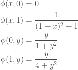
We take the example from (Iserles 2009, chap. 8) where the boundary conditions are:
This has the exact solution
And we can calculate the values of this function on a grid.
> analyticValue :: Monad m => Int -> m (Array U DIM2 Double)
> analyticValue gridSize = computeP $ fromFunction (Z :. gridSize + 1 :. gridSize + 1) f
>   where
>     f (Z :. ix :. iy) = y / ((1 + x)^2 + y^2)
>       where
>         y = fromIntegral iy / fromIntegral gridSize
>         x = fromIntegral ix / fromIntegral gridSize
Let us also solve it using the Jacobi method with a five point stencil and a nine point stencil. Here is the encoding of the boundary values.
> bndFnEg3 :: Int -> Int -> (Int, Int) -> Double
> bndFnEg3 _ m (0, j) |           j >= 0 && j <  m = y / (1 + y^2)
>   where y = (fromIntegral j) / (fromIntegral m)
> bndFnEg3 n m (i, j) | i == n && j >  0 && j <= m = y / (4 + y^2)
>   where y = fromIntegral j / fromIntegral m
> bndFnEg3 n _ (i, 0) |           i >  0 && i <= n = 0.0
> bndFnEg3 n m (i, j) | j == m && i >= 0 && i <  n = 1 / ((1 + x)^2 + 1)
>   where x = fromIntegral i / fromIntegral n
> bndFnEg3 _ _ _                                   = 0.0
We create a function to run a solver.
> runSolver ::
>   Monad m =>
>   Int ->
>   Int ->
>   (Int -> Int -> (Int, Int) -> Double) ->
>   (Int ->
>    Array U DIM2 Double ->
>    Array U DIM2 Double ->
>    Array U DIM2 Double ->
>    m (Array U DIM2 Double)) ->
>   m (Array U DIM2 Double)
> runSolver nGrid nIter boundaryFn solver = do
>   mask    <- boundMask nGrid nGrid
>   val     <- boundValue nGrid nGrid boundaryFn
>   initArr <- mkInitArrM nGrid
>   solver nIter mask val initArr
And put the five point and nine point solvers in the appropriate form.
> s5, s9 :: Monad m =>
>           Int ->
>           Array U DIM2 Double ->
>           Array U DIM2 Double ->
>           Array U DIM2 Double ->
>           m (Array U DIM2 Double)
> s5 n = solveLaplaceStencil n fivePoint 4
> s9 n = solveLaplaceStencil n ninePoint 20
And now we can see that the errors between the analytic solution and the five point method with a grid size of 8 are  .
.
ghci> liftA2 (-^) (analyticValue 7) (runSolver 7 200 bndFnEg3 s5) >>= return . pPrint
  [0.0, 0.0, 0.0, 0.0, 0.0, 0.0, 0.0, 0.0]
  [0.0, -3.659746856576884e-4, -5.792613003869074e-4, -5.919333582729558e-4, -4.617020226472812e-4, -2.7983716661839075e-4, -1.1394184484148084e-4, 0.0]
  [0.0, -4.0566163490589335e-4, -6.681826442424543e-4, -7.270498771604073e-4, -6.163531890425178e-4, -4.157604876017795e-4, -1.9717865146007263e-4, 0.0]
  [0.0, -3.4678314565880775e-4, -5.873627029994999e-4, -6.676042377350699e-4, -5.987527967581119e-4, -4.318102416048242e-4, -2.2116263241278578e-4, 0.0]
  [0.0, -2.635436147627873e-4, -4.55055831294085e-4, -5.329636937312088e-4, -4.965786933938399e-4, -3.7401874422060555e-4, -2.0043638973538114e-4, 0.0]
  [0.0, -1.7773949138776696e-4, -3.1086347862371855e-4, -3.714478154303591e-4, -3.5502855035249303e-4, -2.7528200465845587e-4, -1.5207424182367424e-4, 0.0]
  [0.0, -9.188482657347674e-5, -1.6196970595228066e-4, -1.9595925291693295e-4, -1.903987061394885e-4, -1.5064155667735002e-4, -8.533752030373543e-5, 0.0]
  [0.0, 0.0, 0.0, 0.0, 0.0, 0.0, 0.0, 0.0]
But using the nine point method significantly improves this.
ghci> liftA2 (-^) (analyticValue 7) (runSolver 7 200 bndFnEg3 s9) >>= return . pPrint
  [0.0, 0.0, 0.0, 0.0, 0.0, 0.0, 0.0, 0.0]
  [0.0, -2.7700522166329566e-7, -2.536751151638317e-7, -5.5431452705700934e-8, 7.393573120406671e-8, 8.403487600228132e-8, 4.188249685954659e-8, 0.0]
  [0.0, -2.0141002235463112e-7, -2.214645128950643e-7, -9.753369634157849e-8, 2.1887763435035623e-8, 6.305346988977334e-8, 4.3482495659663556e-8, 0.0]
  [0.0, -1.207601019737048e-7, -1.502713803391842e-7, -9.16850228516175e-8, -1.4654435886995998e-8, 2.732932558036083e-8, 2.6830928867571657e-8, 0.0]
  [0.0, -6.883445567013036e-8, -9.337114890983766e-8, -6.911451747027009e-8, -2.6104150896433254e-8, 4.667329939200826e-9, 1.1717137371469732e-8, 0.0]
  [0.0, -3.737430460254432e-8, -5.374955715231611e-8, -4.483740087546373e-8, -2.299792309368165e-8, -4.122571728437663e-9, 3.330287268177301e-9, 0.0]
  [0.0, -1.6802381437586167e-8, -2.5009212159532446e-8, -2.229028683853329e-8, -1.3101905282919546e-8, -4.1197137368165215e-9, 3.909041701444238e-10, 0.0]
  [0.0, 0.0, 0.0, 0.0, 0.0, 0.0, 0.0, 0.0]


![\displaystyle \boldsymbol{x}_i^{[k+1]} = \frac{1}{A_{i,i}}\Bigg[\boldsymbol{b}_i - \sum_{j \neq i} A_{i,j}\boldsymbol{x}_j^{[k]}\Bigg]](https://s0.wp.com/latex.php?latex=%5Cdisplaystyle++%5Cboldsymbol%7Bx%7D_i%5E%7B%5Bk%2B1%5D%7D+%3D+%5Cfrac%7B1%7D%7BA_%7Bi%2Ci%7D%7D%5CBigg%5B%5Cboldsymbol%7Bb%7D_i+-+%5Csum_%7Bj+%5Cneq+i%7D+A_%7Bi%2Cj%7D%5Cboldsymbol%7Bx%7D_j%5E%7B%5Bk%5D%7D%5CBigg%5D++&bg=ffffff&fg=444444&s=0&c=20201002)

![\displaystyle x_{i,j}^{[k+1]} = \frac{1}{4}(x^{[k]}_{i-1,j} + x^{[k]}_{i,j-1} + x^{[k]}_{i+1,j} + x^{[k]}_{i,j+1})](https://s0.wp.com/latex.php?latex=%5Cdisplaystyle++x_%7Bi%2Cj%7D%5E%7B%5Bk%2B1%5D%7D+%3D+%5Cfrac%7B1%7D%7B4%7D%28x%5E%7B%5Bk%5D%7D_%7Bi-1%2Cj%7D+%2B+x%5E%7B%5Bk%5D%7D_%7Bi%2Cj-1%7D+%2B+x%5E%7B%5Bk%5D%7D_%7Bi%2B1%2Cj%7D+%2B+x%5E%7B%5Bk%5D%7D_%7Bi%2Cj%2B1%7D%29++&bg=ffffff&fg=444444&s=0&c=20201002)


Dear Sir/Madame!
I am a chemistry student and I am interested in computational simulations, so I find your blog great.
But I have a little problem abuot Laplacian stencils, especially the nine-point formula. How can I get these numbers (1, 4, -20)?
Could you help me about this? A good book, or webpage, or something like that maybe help me, (or I hope it will.).
Thank you for your help!
Laszlo Valkai
This are covered in the book by Iserles listed in the bibliography and I thoroughly recommend it. Googling “nine point method” got me this: http://www.physics.arizona.edu/~restrepo/475B/Notes/sourcehtml/node52.html. I will cover it in my book when it finally gets published. Hope that helps.
Thank you! The book you recommended is really great. I will read it! 🙂